Tag: CNC Programming Tips

  • UG NX 1980 Approach, Open Area, and Retract Explained

    πŸ“ Key Takeaways: Master Wang gives a hands-on tutorial, thoroughly analyzing the core parameter settings and practical applications for Approach, Open Area, and Retract in UG NX 1980. This guide helps avoid common machining pitfalls, significantly improving processing efficiency and surface quality. From linear approach to helical, arc, and ramp approaches, and then to retract strategies, each step is combined with practical experience to ensure you learn hard-core knowledge that’s ‘ready for the machine.’

    Introduction: The ‘Tool Tip Dancers’ of Machining Efficiency

    Hello everyone, I’m Master Wang! Today, let’s cut to the chase and talk about the practical aspects of setting up Approach, Open Area, and Retract in UG NX programming. These aren’t just fancy features; they directly impact your machining efficiency and part surface quality. Listen up, this isn’t something you’ll necessarily learn from books, but rather through hands-on experience on the shop floor.

    Part One: Approach Strategies

    Let’s start with the approach. Choosing the wrong approach method can lead to low efficiency, or worse, scrapped parts and broken tools. So, you need to thoroughly understand the nuances here.

    1. Basic Setup and ‘Linear Move’

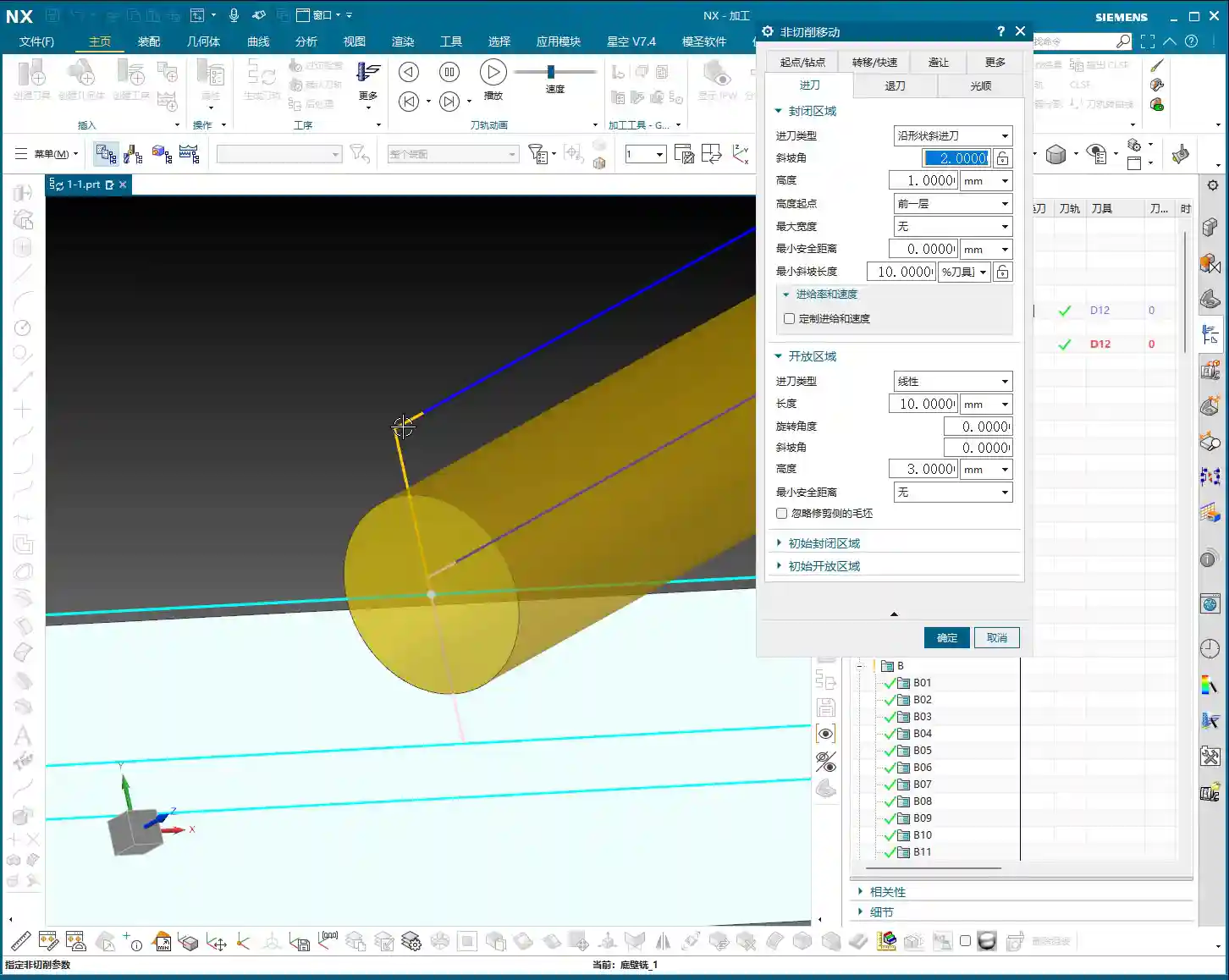
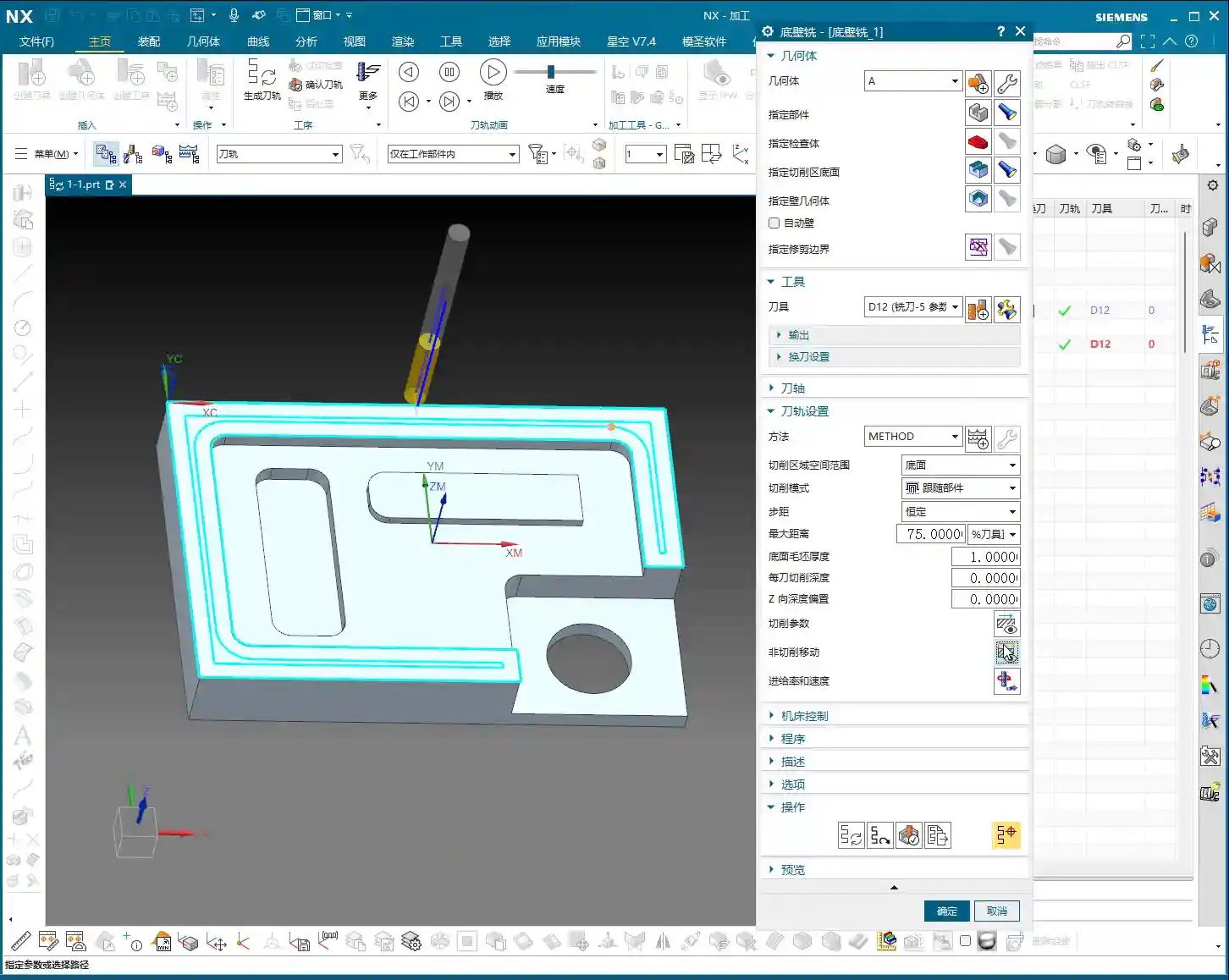
    First, let’s create a standard program and select an appropriate tool, for example, Tool #12. After generating the program, focus on the approach. In the ‘Open Area,’ the default ‘Linear move’ is our most commonly used option. It determines how the tool enters the cutting area from a safe position.

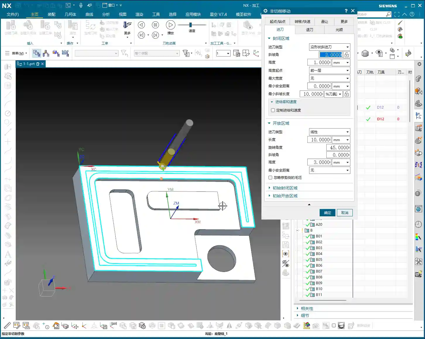
    • Length: This parameter controls the length of the yellow approach line. If you input a value, say 2mm, you’ll see a very short approach line. If you change it to 10mm, the line becomes longer. But there’s a pitfall here: if ‘Extend’ is enabled, the displayed length might not be the actual value you entered. So, to see the true length, it’s best to first disable the ‘Extend’ function. This way, your set 10mm will be the actual 10mm approach length.

    2. Special Approach Method: Same as Closed Area (Helical Approach)

    Besides ‘Linear move,’ there’s the ‘Same as closed area’ option. This is essentially a Helical approach. The tool descends in a helical path, like a drill bit, instead of plunging directly. For situations with pre-drilled holes or harder materials, this can effectively reduce impact and extend tool life. However, in open areas, we use it relatively less often; ‘Linear move’ is more direct and efficient.

    3. Arc Approach

    The ‘Arc’ approach is another common method, where the tool enters along an arc trajectory. This approach is frequently used when performing a Finishing pass on external part contours, especially when finishing walls with a turning tool. An arc approach ensures smooth engagement, reducing tool marks. Of course, in most cases, we still primarily use ‘Linear move.’

    4. Rotation Angle & Ramp Angle

    • Rotation Angle: If you give it an angle, for example, 45 degrees, the tool will not approach perpendicular to the approach line, but rather diagonally. This might be useful in certain special machining conditions, but it’s not commonly used. Just be aware of it.
    • Ramp Angle: For example, setting a 10-degree ramp angle, you’ll notice the tool doesn’t enter horizontally, but ramps down with a slope. This is somewhat similar to the helical effect of ‘Same as closed area,’ also aiming for smoother tool engagement. It also plays a role in specific situations, but it’s not as universally applicable as ‘Linear move.’

    5. Height & Minimum Safe Distance

    • Height: This parameter determines the distance over which the tool will descend at a slow speed before entering the cutting area. For instance, if you input 10mm, the tool will decelerate when it’s 10mm above the part surface and slowly move down. This prevents high-speed plunging. We usually set it to around 3mm, which is sufficient unless there are special requirements. Don’t just rely on software simulation; observe the cutting sparks and listen to the sound to feel confident.
    • Minimum Safe Distance: This is generally a default value, used to ensure the tool maintains a safe distance from the workpiece in non-cutting areas.

    6. Extend & Shrink

    These two parameters are used to lengthen or shorten the yellow approach line. They are not frequently used with ‘Linear move,’ but sometimes come in handy with ‘Arc’ approaches, for example, if you want the arc to be slightly longer or shorter to optimize the cutting path. Of course, we’ll discuss this in more detail later when we cover finishing passes and arc approaches.

    7. Meaning of Open Area and Closed Area

    ‘Open Area’ refers to a region where the tool can freely enter from the outside, such as the side of a part. ‘Closed Area’ refers to a region where the tool is enclosed internally and can only enter through a plunge hole or via a helical approach, etc.

    8. Initial and Final

    Here, ‘Initial closed area’ and ‘Initial open area’ refer to the strategy for the very first tool engagement. For example, if a workpiece has multiple machining faces, the first face might require a specific approach method. We rarely change this parameter; the default usually works well.

    Part Two: Retract Strategies

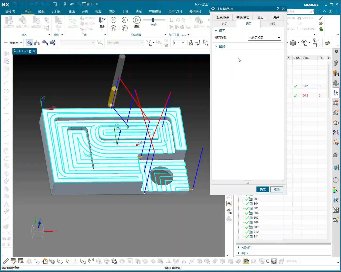
    Now that we’ve covered approach, let’s talk about retract. Retract is actually quite simple; in most cases, we choose ‘Same as Approach.’ This way, the tool exits the same way it entered, maintaining consistency and reducing potential problems.

    1. Direct Retract

    ‘Direct retract’ means the tool lifts vertically immediately after cutting. This method is very abrupt and generally not recommended. Especially in precision machining or when there’s leftover material, direct retract can easily scratch the part surface or increase tool wear. See, that white line is a direct retract. This spot is prone to ‘chatter’; don’t just look at the software simulation, watch the cutting sparks! So, giving it some clearance and retracting smoothly, just like the approach, is the golden rule.

    2. Initial and Final Retract

    Similar to approach, retract also has ‘Initial’ and ‘Final’ options. These control the strategies for the first retract and the last retract, respectively. Again, we generally don’t need to change these; keeping them at their default settings is usually fine.

    Summary: Pitfall Avoidance Guide

    • Distinguish between open and closed areas: This is fundamental for choosing your approach and retract strategies.
    • Maintain consistent approach and retract strategies: In most cases, selecting ‘Same as Approach’ for retract is the most reliable and efficient solution.
    • Use ‘Direct retract’ with caution: Unless you have 100% certainty about the machining conditions, avoid using it to prevent damage to the workpiece or tool.
    • The Height parameter is crucial: Setting an appropriate slow descent distance effectively prevents high-speed plunging, protecting both the tool and the workpiece.
    • Combine theory with practice: Software parameters are static, but machines and workpieces are dynamic. Observe the sparks, sound, and vibrations during machining, and adjust parameters as needed.

    Today, we’ve thoroughly covered these core approach and retract parameters in UG NX. Don’t underestimate these details; a master can guide you, but practice makes perfect. Mastering these will elevate your programming skills to the next level!

    Thank you for watching, see you next time!

  • Master Wang Unlocks UG NX 1980 Machine View Tooling Secrets: Practical Skills & Pitfall Avoidance Guide

    πŸ“ Key Takeaways: Master Wang provides a hands-on guide to leveraging Siemens NX 1980’s Machine View function for precise viewing and management of various tools (face mills, end mills). Learn essential tool parameter settings, quick creation and modification techniques, and how to avoid common programming pitfalls in this practical tutorial.

    Introduction: Tooling Basics Before Programming

    Hello everyone, I’m Master Wang. In our last lesson, we discussed the Program Order View. We’ve already covered those topics, like this specific area here. You don’t need to memorize every single detail of what each function does, but it’s crucial to understand their literal meaning.

    As we delve into programming, you’ll gradually become more familiar with all these various elements, little by little. Eventually, you won’t even need to think about their exact purpose. So, for now, a general understanding is sufficient.

    Core Function: Machine View and Tool Visualization

    Enabling and Understanding Machine View

    This was mentioned before. Let’s look at the option below it, called Machine View. We can simply click on it.

    The main point is that you can see what it means: it displays the Machine View in the Operation Navigator. In essence, it allows you to show the machine and observe how it moves and how the tool operates to machine your part. You can see all the toolpaths and movements.

    However, for our initial learning phase, we haven’t even created a program yet, so this feature isn’t immediately useful. If you want to use it, you would go to Edit, then ‘Load Machine from Library’ to find many different machines. But we won’t go into that for now.

    Understanding the Tool List: Templates and Customization

    What we need to discuss are the items below. You can scroll down; these can be dragged down further. What do all these items mean at the bottom? I believe many of you might already have some understanding and will grasp it quickly.

    This entire section contains all of our tools. Where are our tools located? They are all placed here on the side.

    Why are these tools here? It’s because of the template I created at the very beginning, remember? That template.

    If you wish to add or delete these tools yourself, you need to go into that template to perform the addition or deletion.

    How do you do it? Please refer to my ‘Master Wang’s Template’ tutorial; there’s a ‘Programming Template’ section within it. Go there to see how it’s created.

    In-Depth Analysis of Tool Parameters

    Face Mill E100 Example: Diameter, Length, and Effective Length

    Let’s take a look. The creation method is quite simple.

    Let’s examine what this means. For example, the first one is E100. The meaning of E100, frankly, refers to its diameter.

    Look, if sometimes it doesn’t display, you can click somewhere else, then click on this E100 again, and the tool will reappear.

    The diameter is 100, meaning the entire diameter of this tool is 100 mm.

    At this point, we can double-click to open it, or right-click and ‘Edit’, both work. I’m used to double-clicking to open it.

    Double-click to open. After opening, let’s look at this area.

    The diameter is 100. Clearly, this tool’s diameter is 100 mm. The bottom diameter is 0. These others are also 0; we can ignore them.

    The length is 75 mm. Simply put, the total length of this tool is 75 mm. And the effective length is 50 mm, which means the distance from this point to this point is 50 mm.

    Of course, as you all know, what E100 means is that it’s a face mill, a face mill with a 100 mm diameter.

    Its bottom radius is 0, which means it should typically be E100 R0.8. Usually, the inserts for these tools have a small corner radius of R0.8. So, it’s a tool like E100 R0.8. Why did I set the bottom corner radius to 0? We’ll discuss that later when we get to programming. For now, just understand what this tool represents.

    This face mill has a total length of 75 mm and an effective length of 50 mm.

    You might ask, how can the effective length be 50 mm? Because for insert tools, the insert itself isn’t 50 mm long. The point here is that we can give it an approximate value. You don’t need to create it to be exactly identical to the physical tool. We only need to create the approximate size of the tool, and that’s sufficient.

    Tool Positioning and Machining Simulation

    Now, by default, whenever we open the tool, it will appear in this position. We can click and hold the left mouse button to drag it, or simply click on a specific spot on the screen to place the tool there.

    What is this actually for? Simply put, we can place it, for example, approximately here. Then we can check if a single pass of this tool can cover the entire area. This is the edge, and this is the edge. If it starts cutting from here, moves along, and then comes over, can one pass cover it? Clearly, it can. A 100 mm tool can cover this area.

    Okay, when we reach this position, there’s a significant amount of material here. You also know what this means. It means our tool is too large to machine this corner radius. In such a situation, we would definitely need another type of tool to perform corner cleanup. Just understand this concept.

    We can’t machine all the way to this point, right? If we did, we’d be overcutting this area.

    The purpose of this is simply for reference. It allows us to check if the tool is large enough, or if it’s suitable, if we can use this tool. Just take a look, a rough look. But for the final selection, you also need to check what tools you actually have available.

    You can click anywhere; clicking here or on that corner, both are fine.

    Alright, so this is about how to change or view our tools. Roughly, there’s also the length and effective length. That’s good. Let’s move on.

    Quick Tool Creation and Modification (Critical Pitfalls)

    E-Series Face Mills: Copying, Renaming, and Parameter Modification

    For example, now we have E59, E90, E80, E63, E40. All of these are insert tools (face mills with removable inserts). Any tool starting with ‘E’ is typically an insert-type tool. E25, E21, E20, E17, E16.

    For instance, let’s say we want to create an E15 tool. How do we create it?

    Right-click, Copy. Then directly click Paste. Good.

    Now, this tool and the original one are actually identical. It’s just like copying and pasting any other item, like a folder or anything else. The copied and pasted items will definitely be identical.

    We need to modify the pasted tool. Right-click. Why is there English at the end? Because their names cannot be duplicates.

    For example, for E17, just change the ‘6’ to ‘7’, and press Enter. See, now you have an E17 tool, right?

    Oh, for E15. Right-click, Rename. We’ll take this position, you can drag it a bit, and change it to ‘5’. Okay.

    Can it be used now? We copied it and changed its name to E15. Is this correct? Absolutely not!

    Although its name has been changed to E15, this tool is still a 16 mm tool. Everyone, please, please, please remember this: just renaming the tool’s display name to E15 does not make it an E15 tool. That’s impossible. You must double-click to open it, then go to the Diameter field and enter 15. Good, then press Enter. That’s all. Of course, there are other parameters like tool holder, etc., but for now, we don’t need to worry about them. We just need to make sure the diameter is correctly set. The length and effective length have already been discussed.

    Right-click, OK. Only now is this tool truly an E15 tool. Double-click to open and check again. 15, correct. OK.

    R-Corner Radius Tools: Distinguishing E90R0.8 and E63R6

    Let’s look at the E90 R0.8 below. Actually, this one and the E90 are quite similar. But the R0.8 indicates that at this position, there is a small corner radius. This position has an R0.8.

    Why are these two types of tools so similar? It’s simply my personal habit for future programming; I might need both. We’ll discuss that later. For now, there’s no need to explain it so thoroughly; we just need to understand what these tools mean.

    We also have E63 R6. Everyone knows this type of tool, right? It’s an E63 face mill with an R6 insert. This is an R6 insert, quite large, a round type of insert.

    E63 R0.8 is a square-ish insert.

    These are all self-explanatory, and the differences are quite clear.

    D-Series End Mills: Similarities and Differences with E-Series

    For example, for an E25 R5 tool, we copy it, and then paste it.

    Suppose we want to create an E26 R5. Just create a random one.

    Rename. The first step is to rename it. E26 R5. Delete all the English characters at the end, then press Enter.

    At this point, we double-click to open it. E26 R5. We don’t need to change the ‘R’ value.

    Let’s say, for example, you don’t want to confirm directly now. Suppose you realize you made a mistake with this tool in your work. You can double-click to open it. For example, if you want to create an R4 tool. You change it to 4. You must press Enter. If you change it to 5, you have to press Enter. When you preview this ‘R’ value, for example, if you input 1, press Enter. Okay, now this position is 1. You must press Enter; it’s a habit. Enter. Okay, Enter, Enter.

    R4, Enter.

    Don’t worry about the effective length or anything else; just click OK. But you must rename it from ‘5’ to ‘4’, because you’ve already changed the internal parameters to E26 R4, so the external name also needs to be updated. OK.

    This is a quick way to create a tool. This method of creating tools, I think, is quite convenient; you just copy and paste.

    All tools starting with E are typically insert tools (face mills).

    Now, what about tools starting with D? These are actually end mills. They are not insert tools, meaning they can machine with their side cutting edge as well. I believe everyone has seen this type of tool in the machine shop. You’ve definitely seen them.

    D35 R3 means a 35 mm end mill with an R3 corner radius, very clear. D14 R1.5 means a 14 mm end mill with an R1.5 corner radius.

    For example, how do you create this? The creation method is exactly the same as what we just did.

    Summary: Pitfall Avoidance Guide

    Listen up, Master Wang emphasizes again:

    1. Name vs. Parameters: In Siemens NX, renaming a tool’s display name (label) does not automatically change its actual machining parameters! You must double-click to open the tool properties, manually modify core parameters like diameter, length, and corner radius, then press Enter to confirm, and finally click OK for the changes to take effect. This is the most common pitfall for beginners.
    2. The ‘Approximate’ Rule for Effective Length: For a tool’s ‘effective length’ (or cutting length), especially for non-standard tools or face mills, providing an approximate value that meets machining requirements is sufficient in the model. There’s no need to demand 100% exact match with the physical tool. The software model is mainly for visual simulation and toolpath calculation.
    3. Machine View for Visual Verification: Use the Machine View to visually check if the tool’s size is appropriate, if it can cover the machining area, and if there’s any risk of overcutting. Don’t just rely on software simulation; you need to envision the cutting sparks! While this is virtual, this way of thinking is fundamental to practical machining.
    4. Significance of Corner Radius (R-Value): Understand the meaning of the R-value in tool names (e.g., R0.8, R6). It represents the corner radius of the tool’s cutting edge. Different R-values correspond to different insert shapes and machining characteristics (sharp corner, rounded corner), which are crucial for corner cleanup and contour milling.
    5. E-Series vs. D-Series: Familiarize yourself with common tool prefix conventions in Siemens NX. Typically, ‘E’ series often refers to face mills / indexable face mills (Face Mill) with replaceable inserts, suitable for roughing flat surfaces. ‘D’ series often refers to end mills / ball nose end mills (End Mill/Ball Nose), commonly used for side milling or finish contour milling.
    6. Importance of Templates: Your tool library should be built upon standard templates. The initial tool list comes from your programming template. Learning to manage and customize templates can greatly improve efficiency.