📝 Key Takeaways: Hello everyone, this is Master Wang. Last time, we covered roughing. This time, the focus is on finishing rotary parts. From side walls to bottom surfaces, and then to root corner cleanup, I’ll walk you through programming efficient, high-quality toolpaths using Siemens NX. I’ll share practical tips you won’t find in textbooks, such as how to optimize tool retractions, prevent overcutting, and tackle various machining challenges. My goal is for you to not just program, but truly understand the machine and the process.
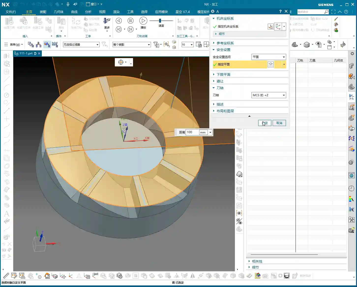
Step One: Finishing Side Walls and Bottom Surfaces – Refined Application of Depth Profile Milling
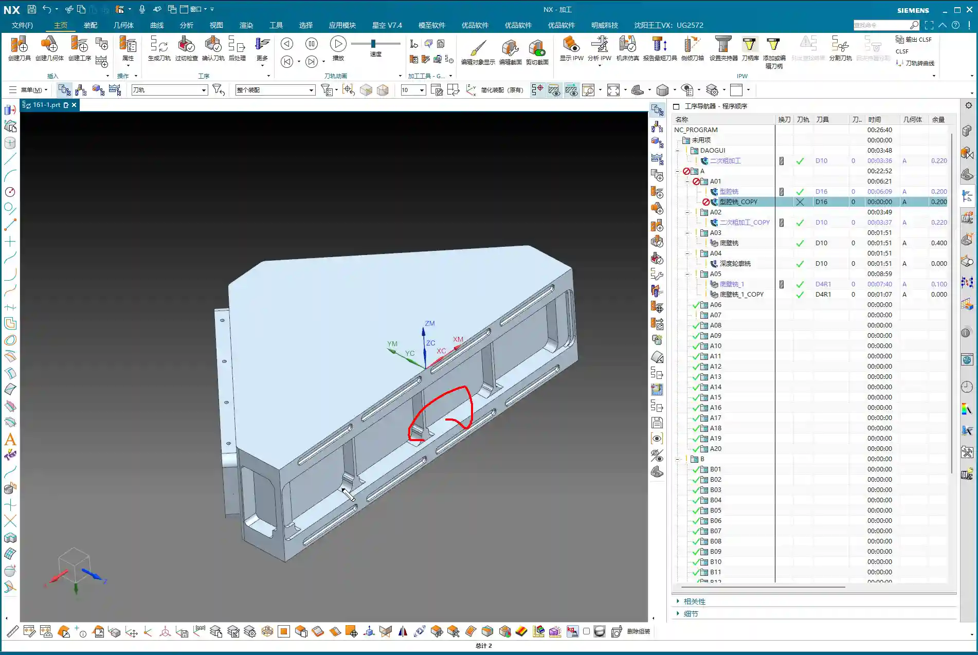
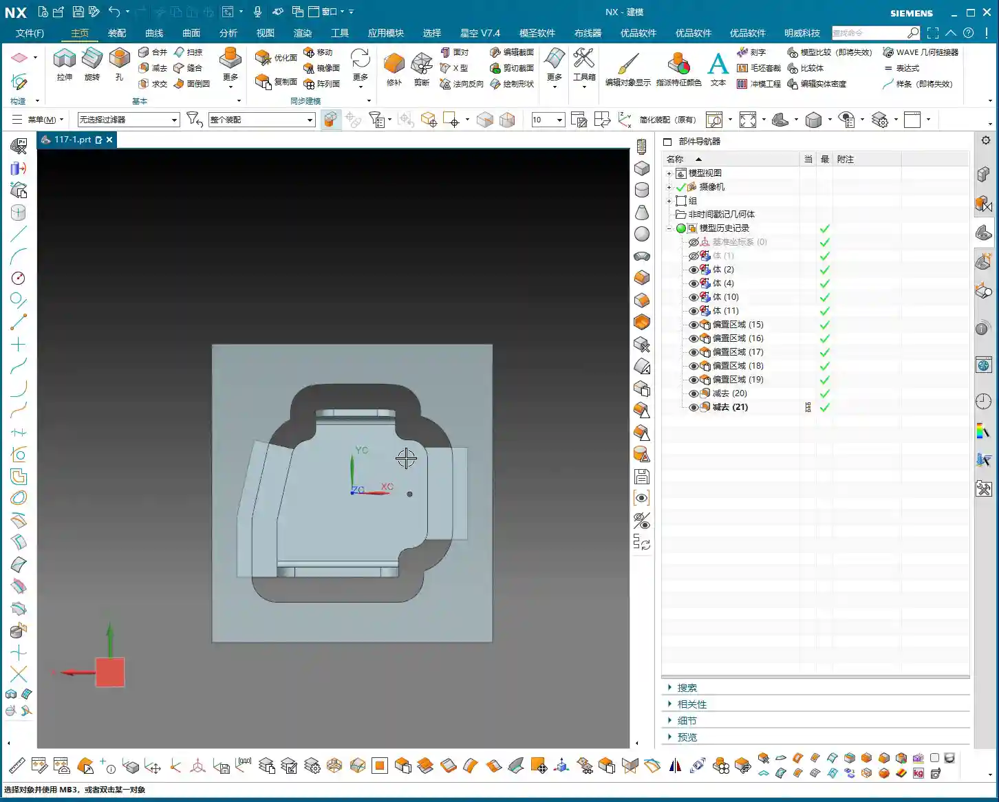
Listen up, last time we thoroughly covered roughing and semi-roughing. This time, we’re heading straight into finishing, focusing on the part’s side walls and bottom surfaces. Especially that bottom area – we might have left some stock last time, but this time it needs to be completely cleaned, leaving no blind spots.
Practical Tool Selection and Machining Area Definition
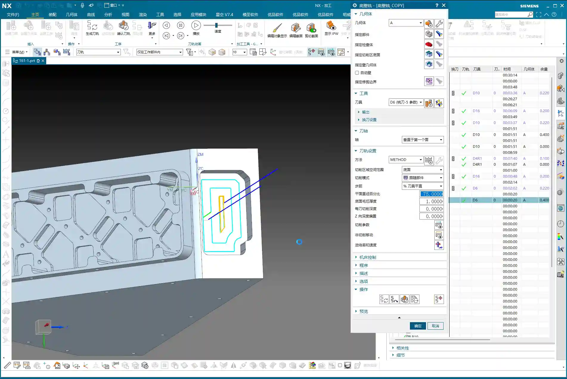
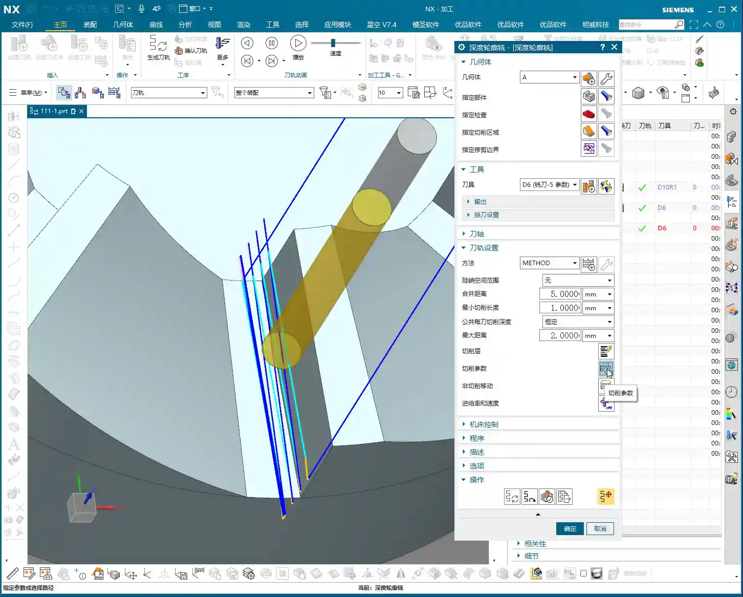
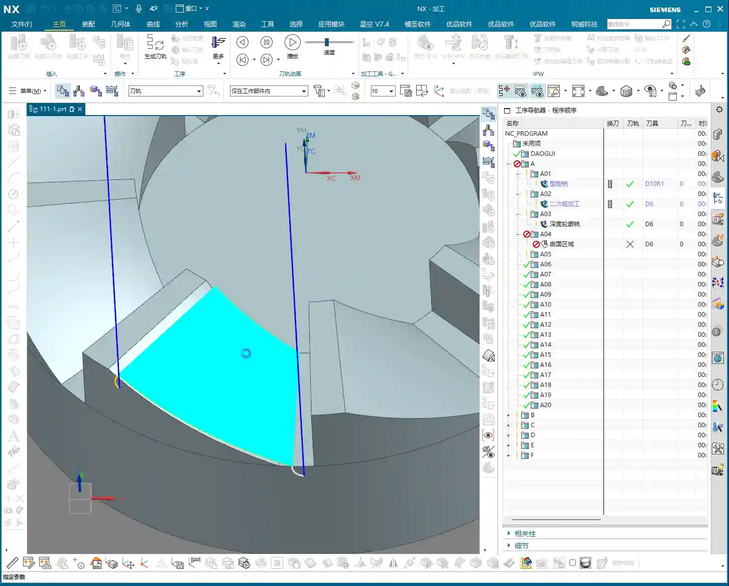
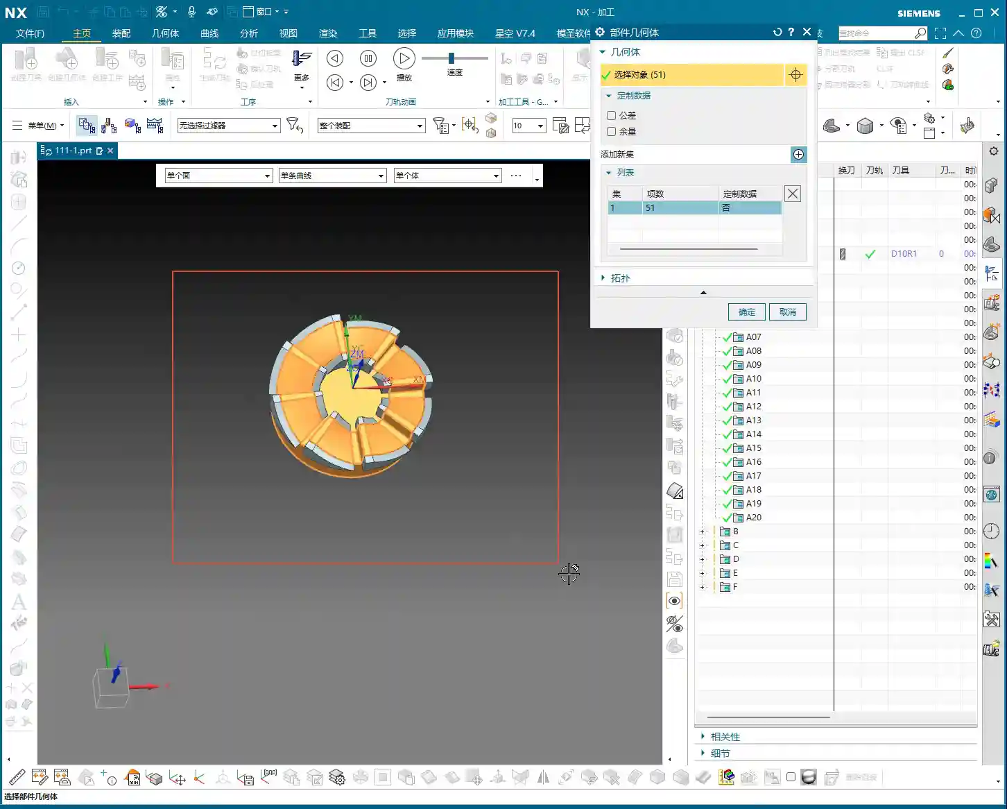
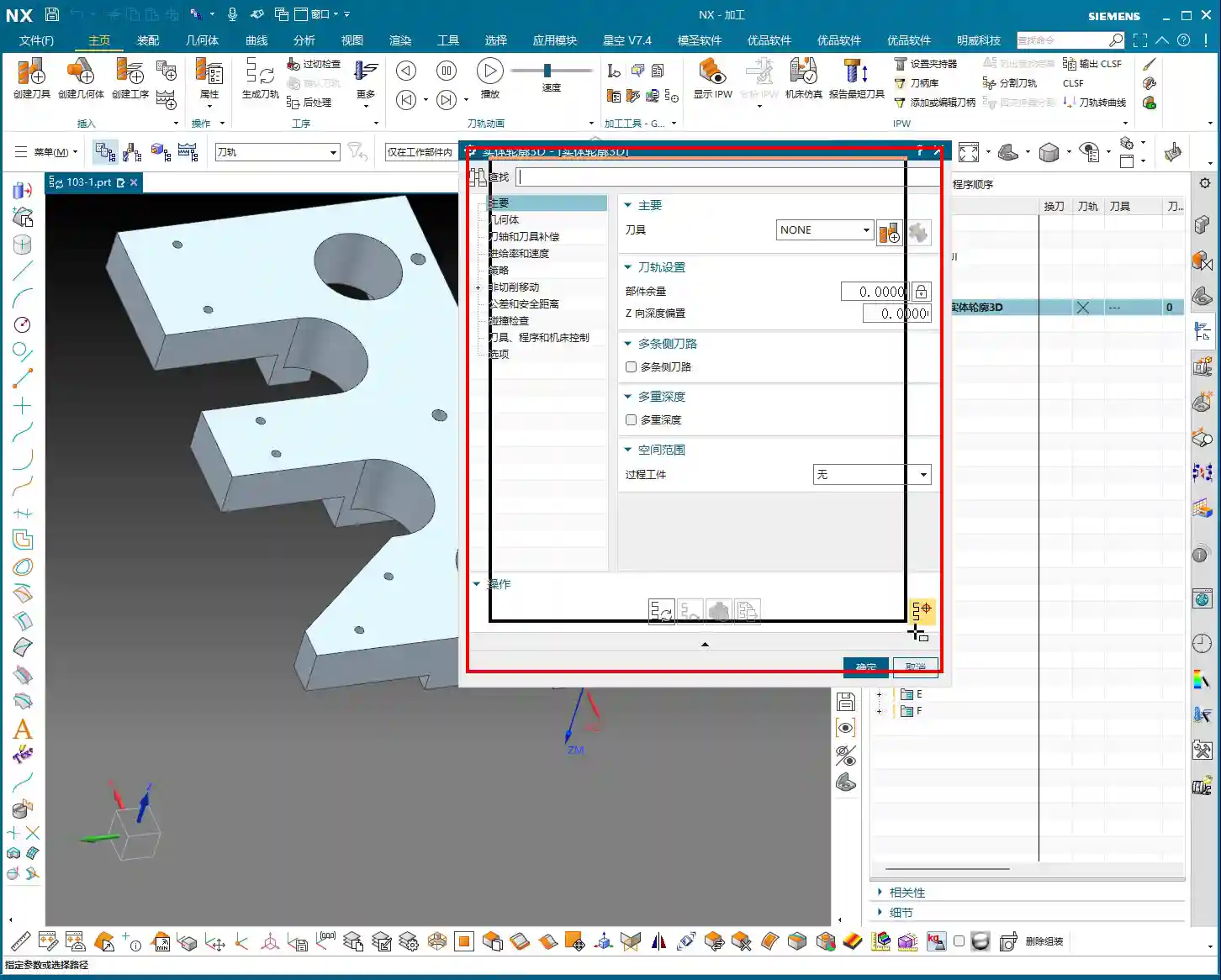
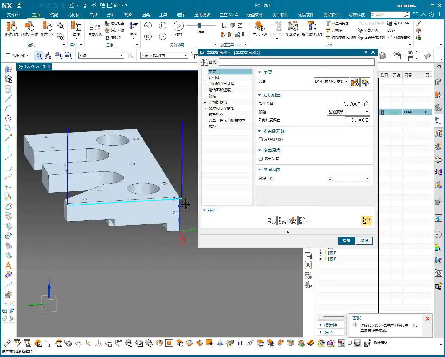
First, open your NX software. We’ll select a “Depth Profile Milling” operation. For tooling, we’ll directly choose our commonly used D6 flat end mill; this tool will handle the corner cleanup and side walls. As for the machining area, you can initially box-select the entire part; that’s fine, we’ll precisely define it later.
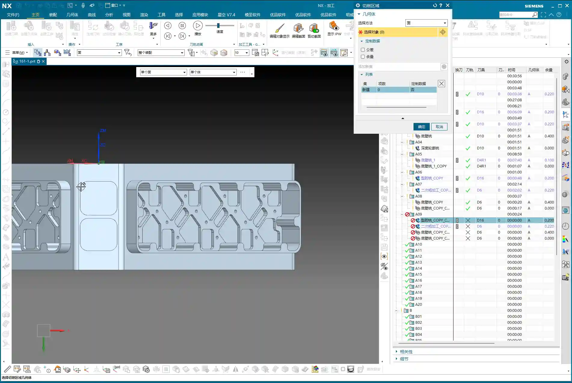
Hold on, what we need to do is specifically select these two areas: the side walls and the bottom surface. Remember, precision selection is better than broad selection. This avoids many unnecessary issues and computational load, improving program generation efficiency.
Depth of Cut and Multi-Pass Strategy
This program is primarily for finishing passes on the side walls. As I mentioned last time, the stepover for side walls should be tighter to achieve a smoother finish. For the bottom surface, we’ll machine down to a depth of -18mm. Of course, to be safe, you can adjust it slightly shallower, say -17mm, to leave a bit of stock for the final finishing pass.
Here’s the critical point: that last 1 millimeter (approx. 0.04 inch) of stock on the bottom surface (for example, from -17mm to -18mm) – you absolutely cannot take it off in a single pass! Doing so risks chatter or tool breakage, and the resulting surface won’t be flat. We need to split it into multiple layers, for instance, taking 0.3mm (approx. 0.012 inch) per Depth of Cut (DOC). By cutting in two to three layers this way, the cut will be stable, and the finish will be superior. Don’t just rely on software simulation; pay attention to the cutting sparks and the actual forces on the tool!
Additionally, the top 5 millimeters (approx. 0.2 inch) of the side wall should also receive extra finishing passes to improve its flatness. During the finishing pass stage, we won’t leave any stock; it’s a direct one-pass finish.
Cutting Parameters and Safety Strategies
For the cutting order, we’ll select Depth First. As for stepover, a linear cut at 55% or 60% is fine; this depends on your tool’s strength and material properties. However, I typically disable extension to avoid unnecessary toolpaths.
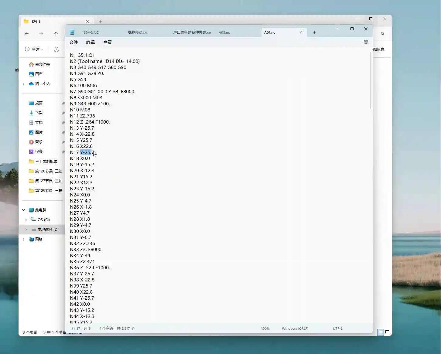
The program has generated, and the cutting depth control is fine. But look at this rapid move – it plunges directly into the side wall! This is unacceptable! A machine tool isn’t a computer simulation; this kind of move risks a collision. At best, you’ll scrap the tool and workpiece; at worst, you’ll damage the machine!
Therefore, we need to go into “Non-Cutting Moves” and modify the rapid transfer. For safety, retract to the stock surface; that 3-millimeter (approx. 0.12 inch) height is acceptable. This provides sufficient safe retraction space for the tool. This is a crucial safety procedure, remember that!
Here’s another trick: if the toolpath keeps failing to generate or takes excessive detours, it’s likely because a previously selected face is restricting it. Just select the bottom surface and the two side walls; don’t select the upper faces, let the tool move freely! Simplifying your selections often resolves major issues.
Finally, overcut checking is fundamental! Don’t assume everything is fine just because the program generated. One overcut can undo all your previous work, or even scrap the part.
Step Two: Corner Cleanup and Angled Surface Finishing – Surface Drive and Guide Curve
All right, the side walls and bottom surface are finished. Next, let’s address the root area of this part. After corner cleanup, we also need to perform contour milling on this angled surface. What command do you think is suitable?
Corner Cleanup Toolpath: Surface Drive is the Correct Approach
Some might think of using a “Guide Curve” for corner cleanup. But listen up: Guide Curve only supports ball end mills. How can a ball end mill perform corner cleanup? It simply can’t clean effectively! If the root has a sharp corner or small radius, a ball end mill can’t reach the bottom. Others might suggest using “Streamline” offset lines, which can also work, but that’s too much hassle—offsetting lines, selecting them—it’s highly inefficient!
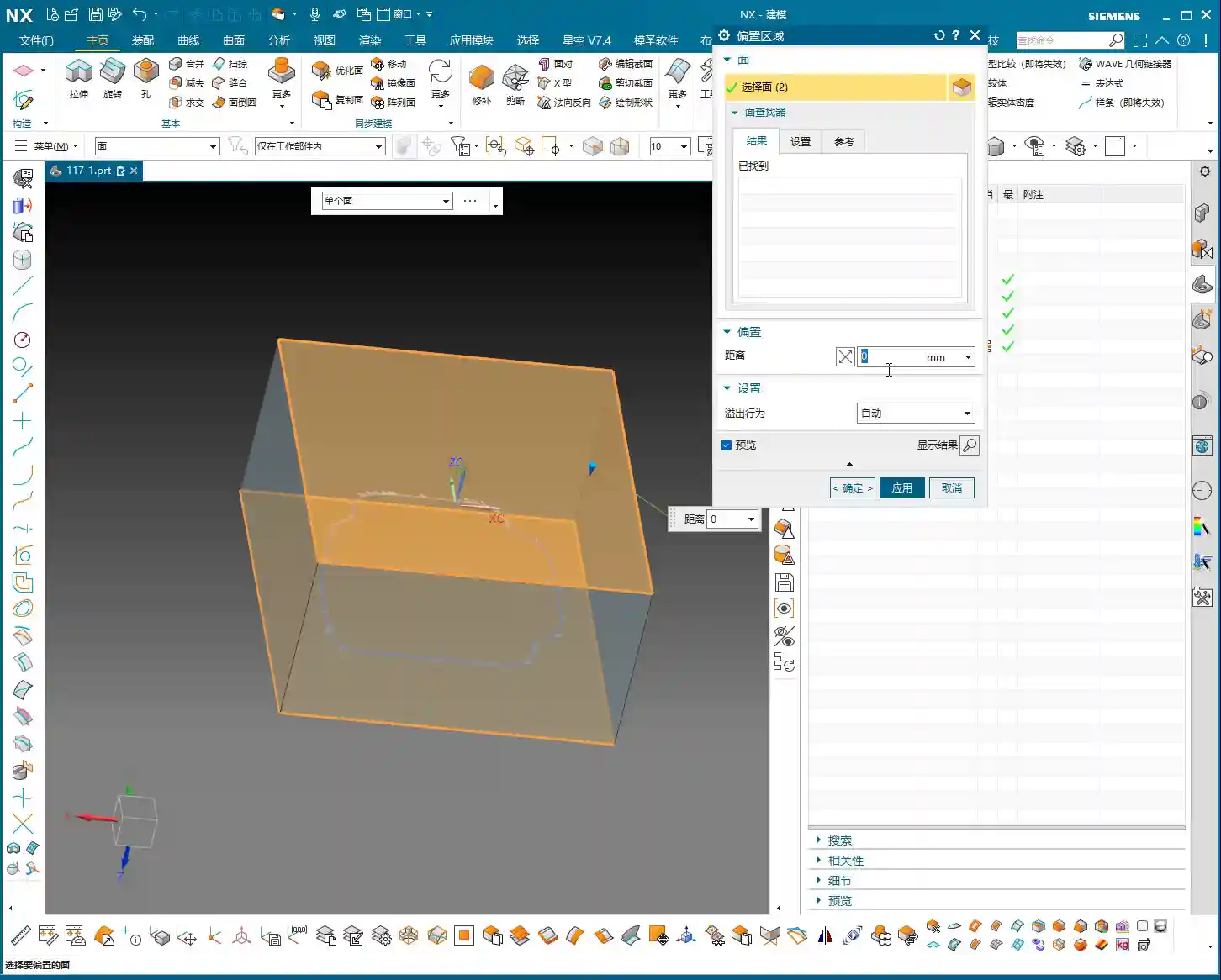
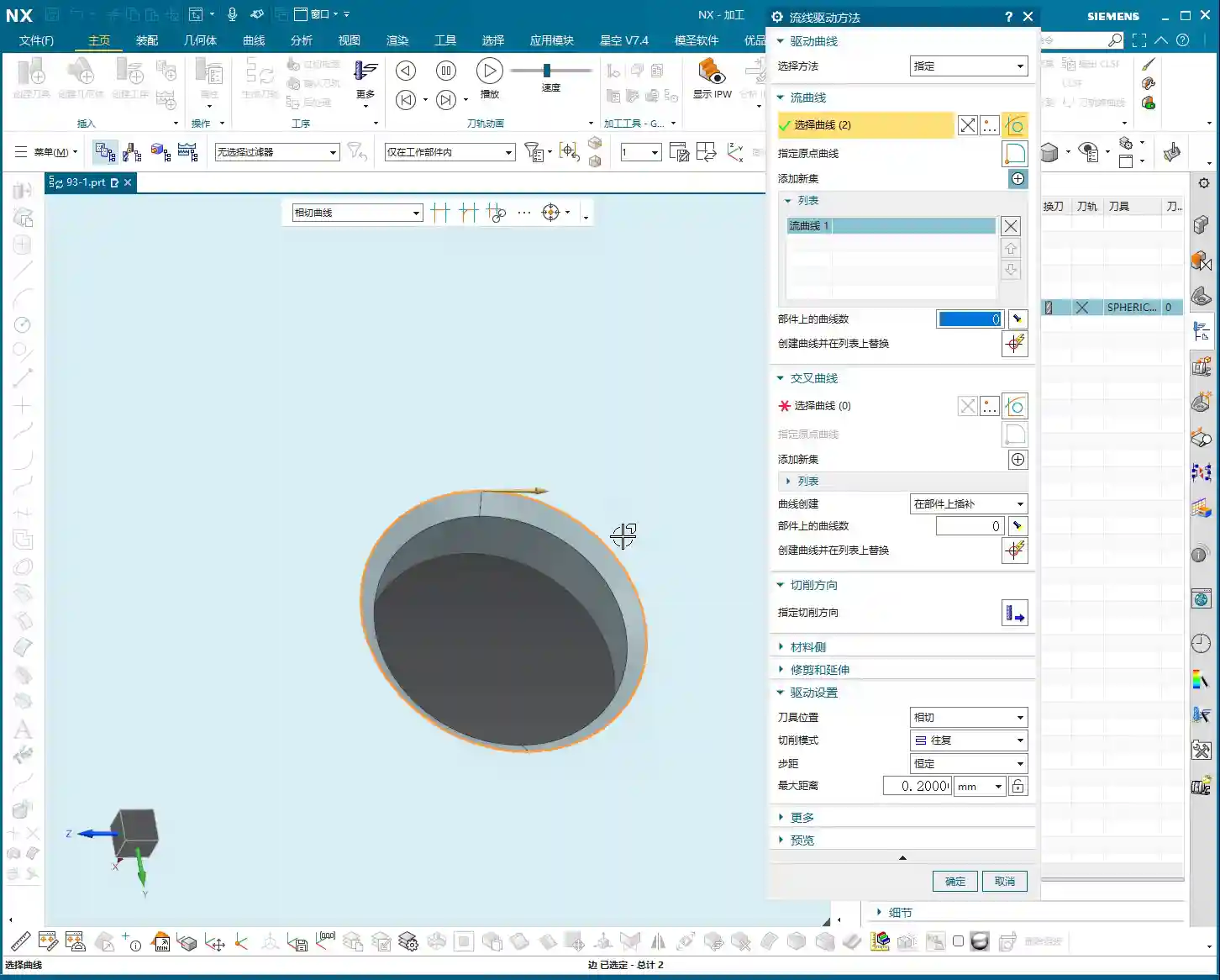
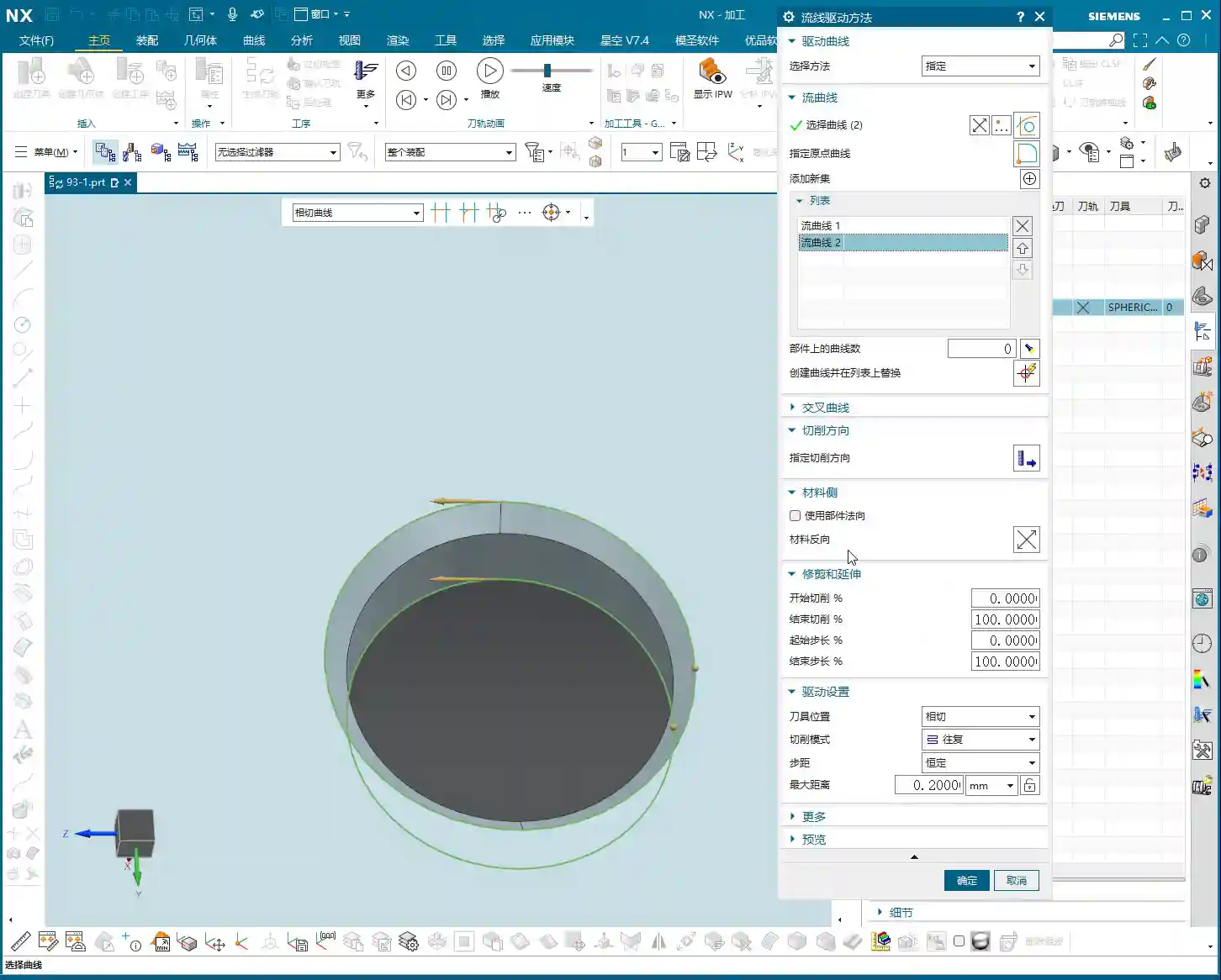
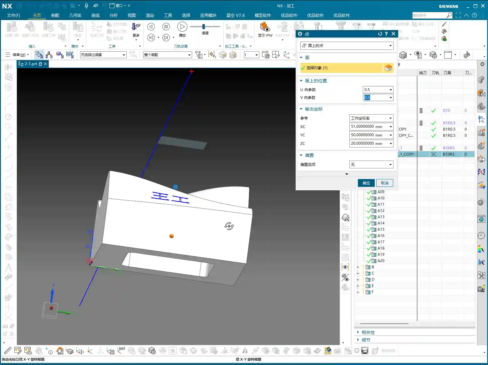
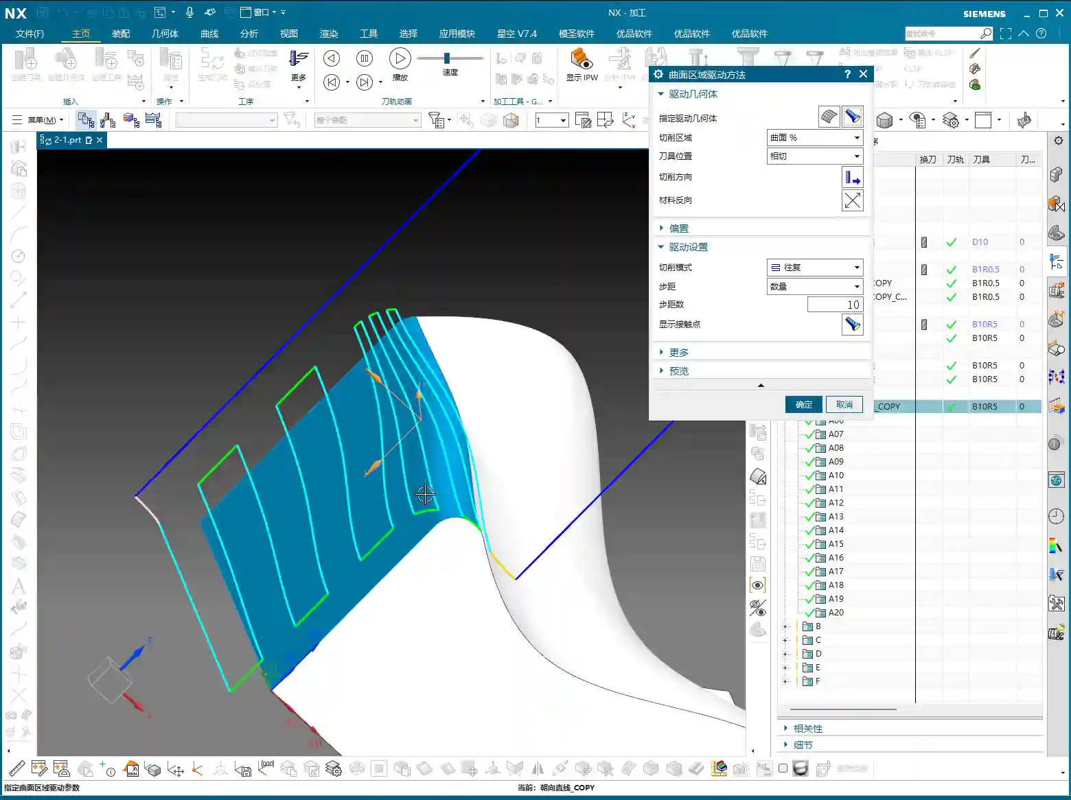
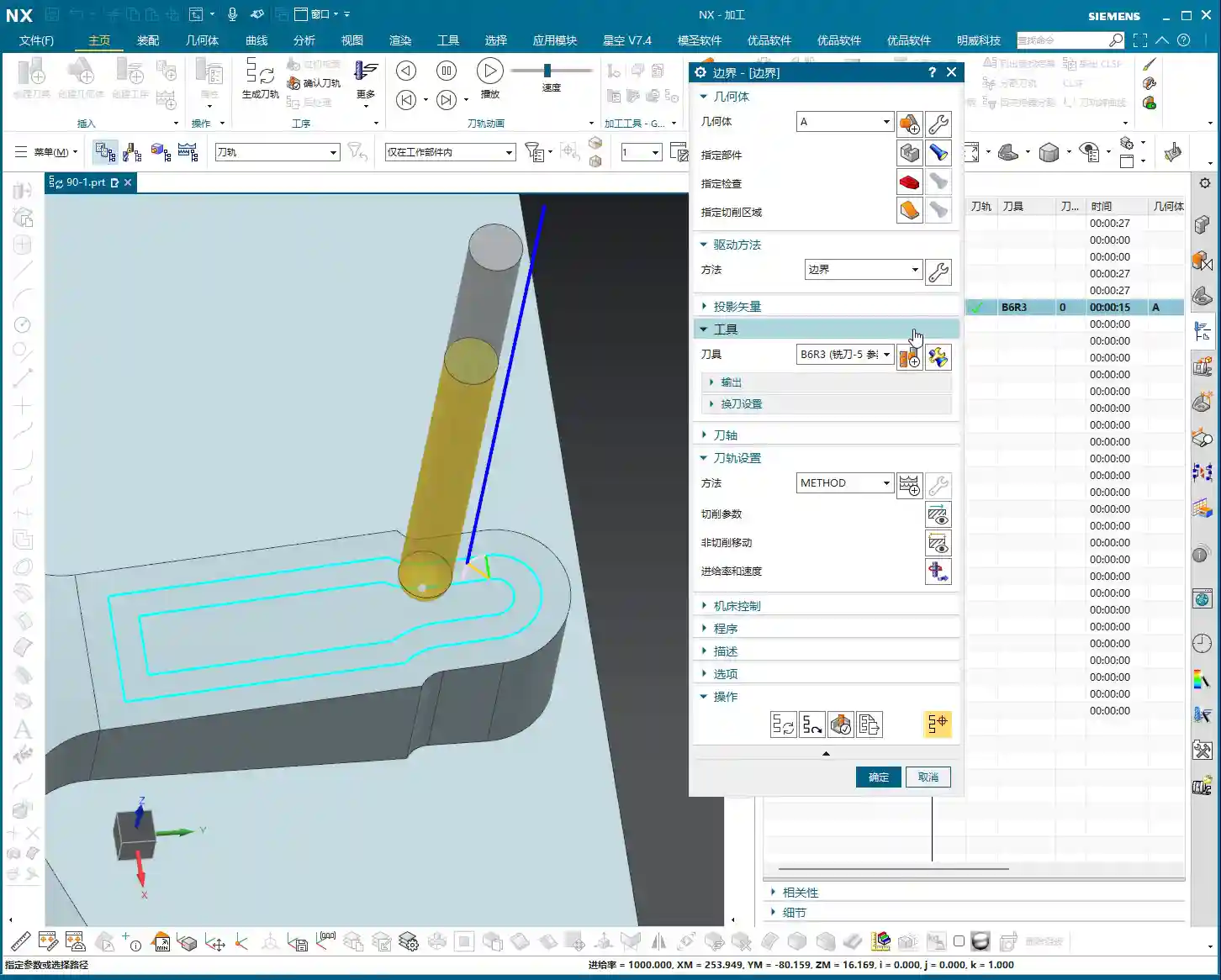
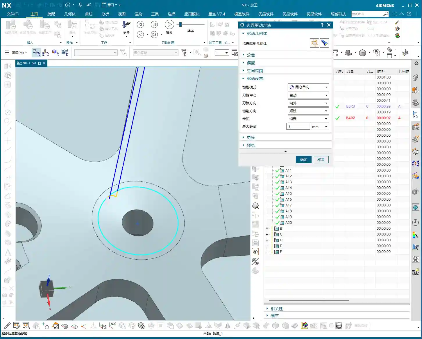
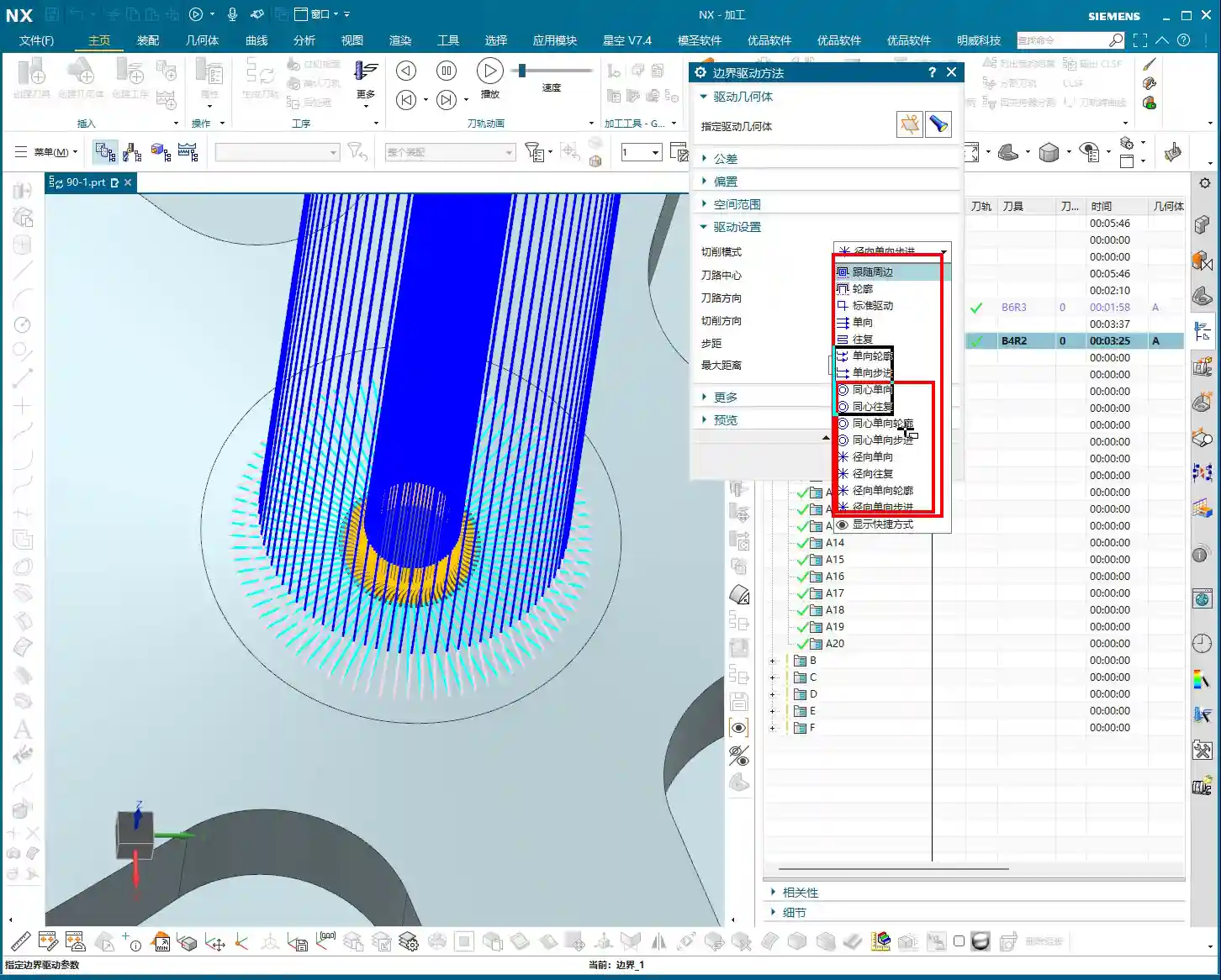
So, the most direct and effective method is our Surface Drive. This command is specifically designed for this! We’ll still use our D6 flat end mill. This time, there’s no need to select a machining area; just select the “drive face.”
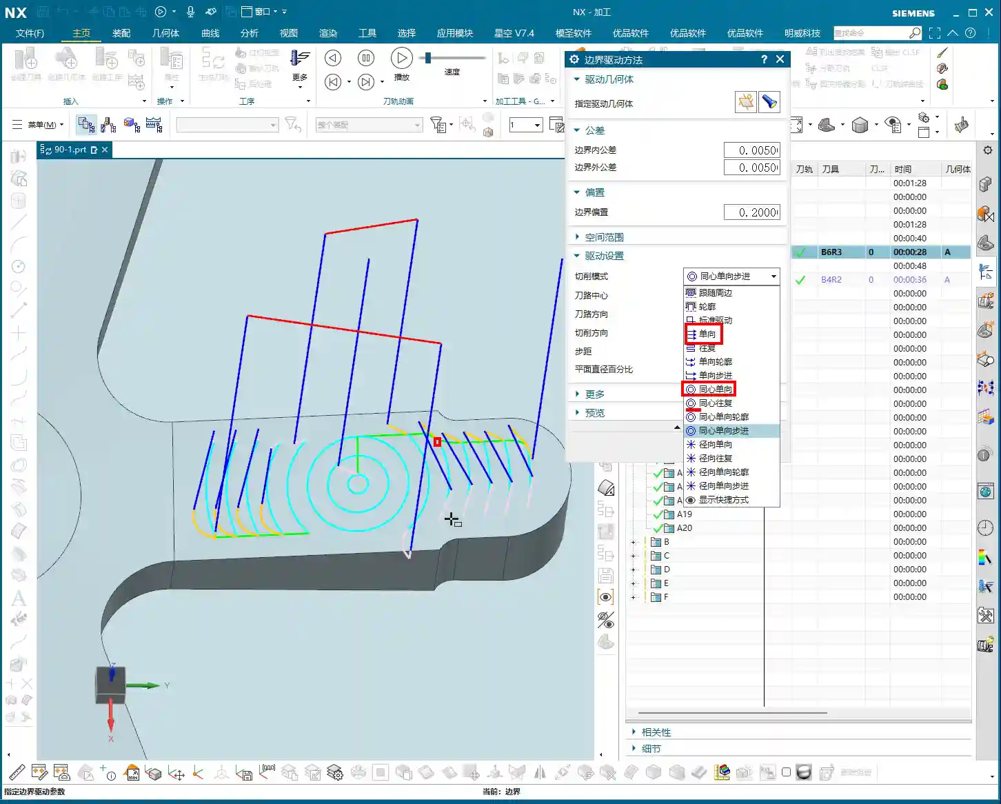
Pay close attention to the cutting direction; we’ll set it to Material Reverse and use Zigzag machining for higher efficiency. For corner cleanup, a 0.1-millimeter (approx. 0.004 inch) stepover! When performing corner cleanup with a D6 flat end mill, a small stepover is crucial for a clean cut; otherwise, the finished surface won’t be flat, and all your effort will be wasted! Remember, finishing passes require attention to fine details; no need to change tolerances, just calculate the toolpath directly.
Toolpath Trimming: Precise Control of Machining Area
The program has generated, but it’s currently cutting from top to bottom, and we only need that small root area at the bottom. This is where the Trimming function comes in – listen up, this is key to boosting efficiency!
Within “Cutting Area,” locate “Surface Percentage.” See, we initially clicked this arrow (pointing at the direction), so Start Trim calculates from the top, and End Trim goes to the bottom. We need to shorten it to only machine the root area, which means modifying Start Trim. For example, changing it to 97% will make it cut only the very last portion. You’ll need to experiment a few times to find the appropriate percentage until the toolpath precisely covers the root area. This all comes from experience; you have to get hands-on.
Exploration: Applying Guide Curves and Optimizing Retract Moves
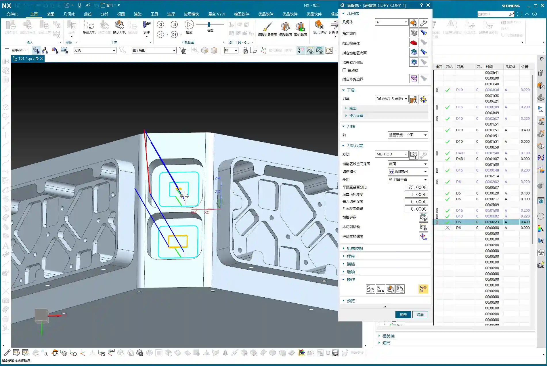
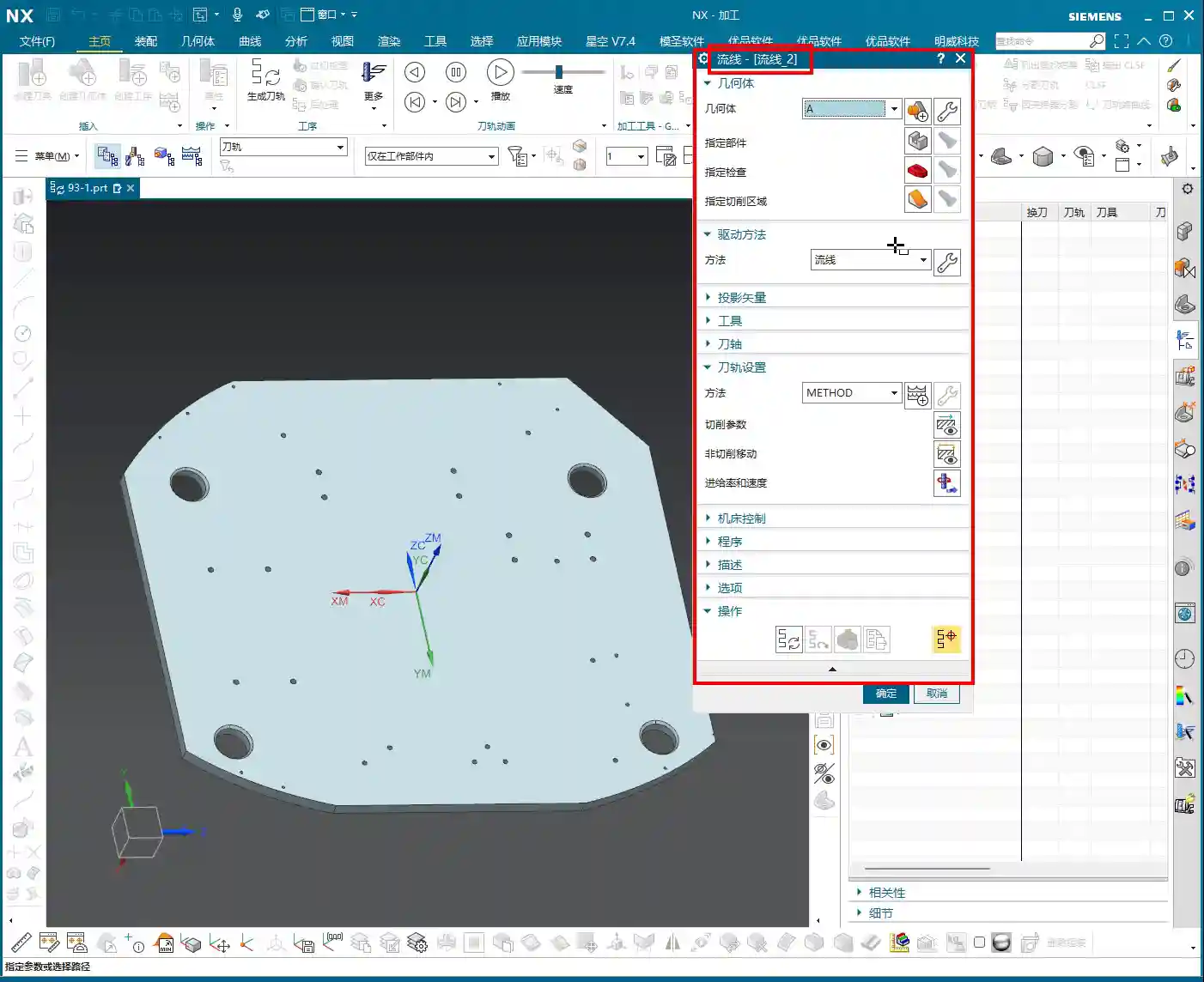
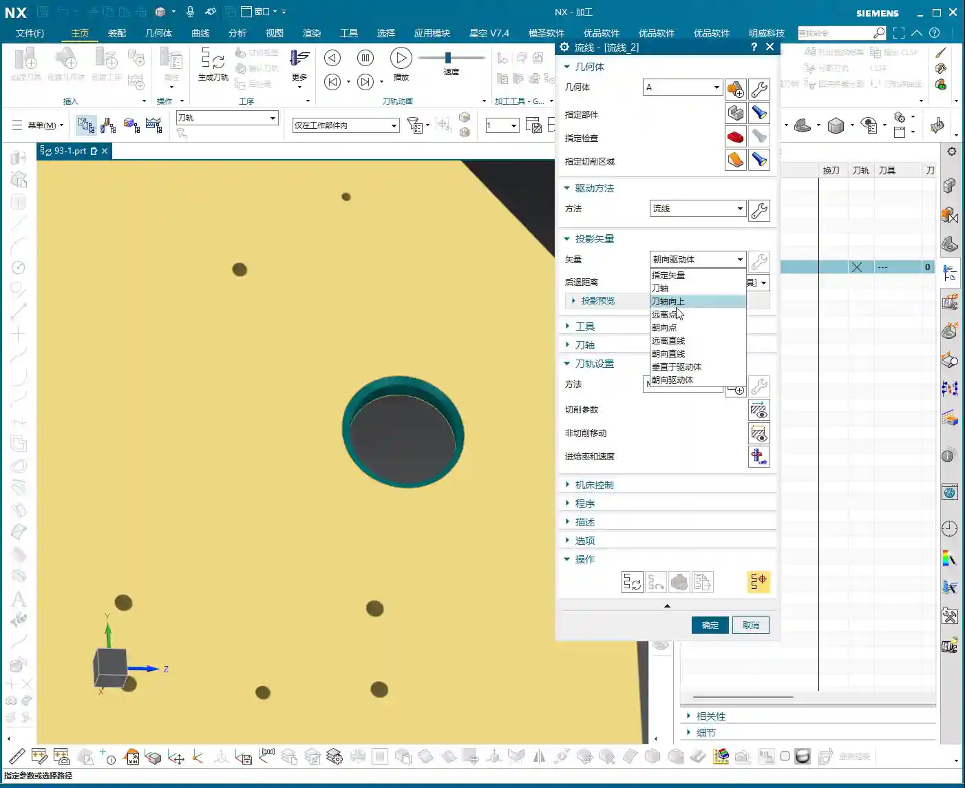
While Surface Drive works well for corner cleanup, to broaden your understanding of different methods, we can also try using a Guide Curve to machine this angled surface. You might not have used it much before, so let’s get some hands-on practice. Honestly, for machining such surfaces, any command will do – Contour Milling or Surface Drive, both are viable. The key is to find what’s best for the current situation; don’t fret, nothing is too difficult!
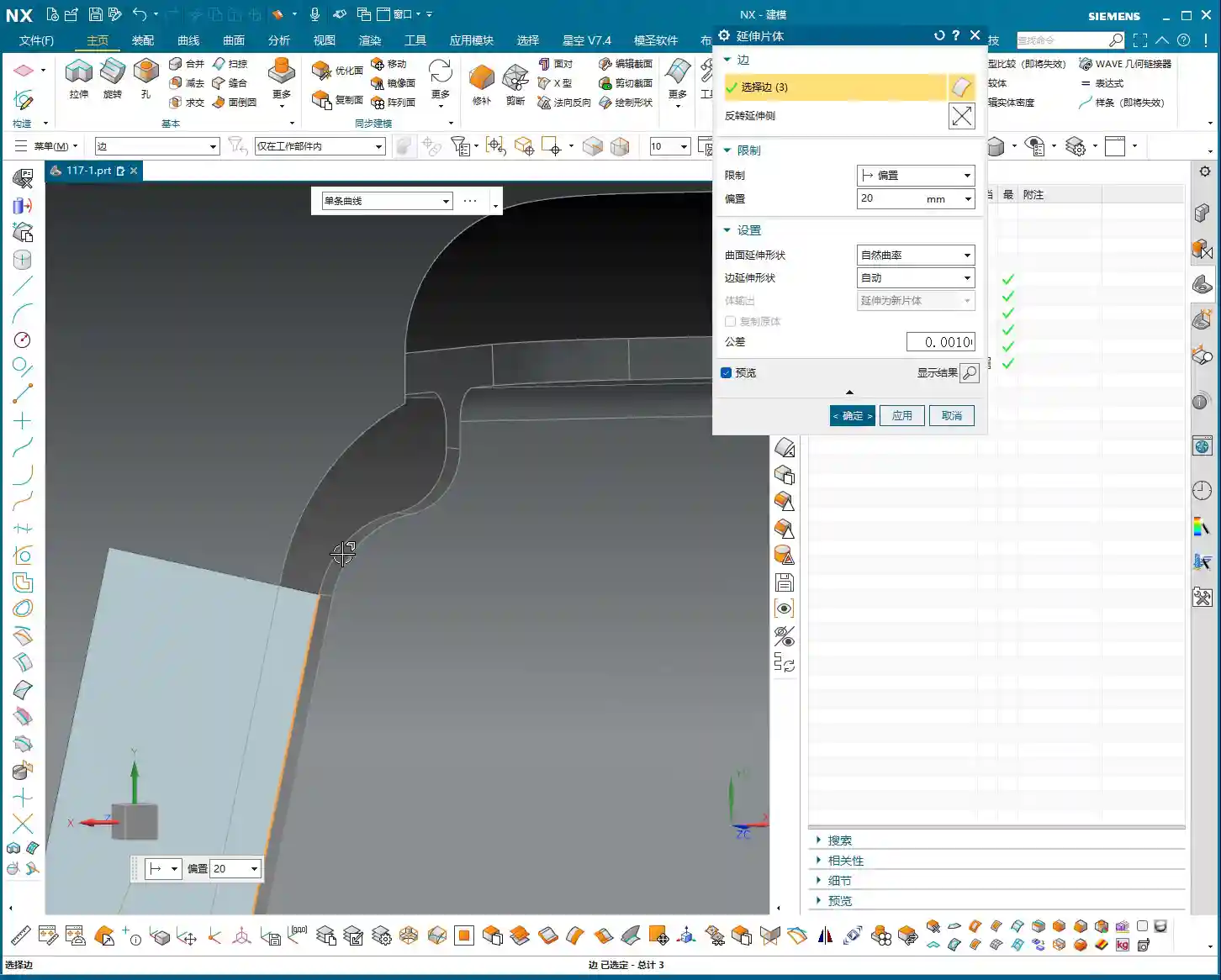
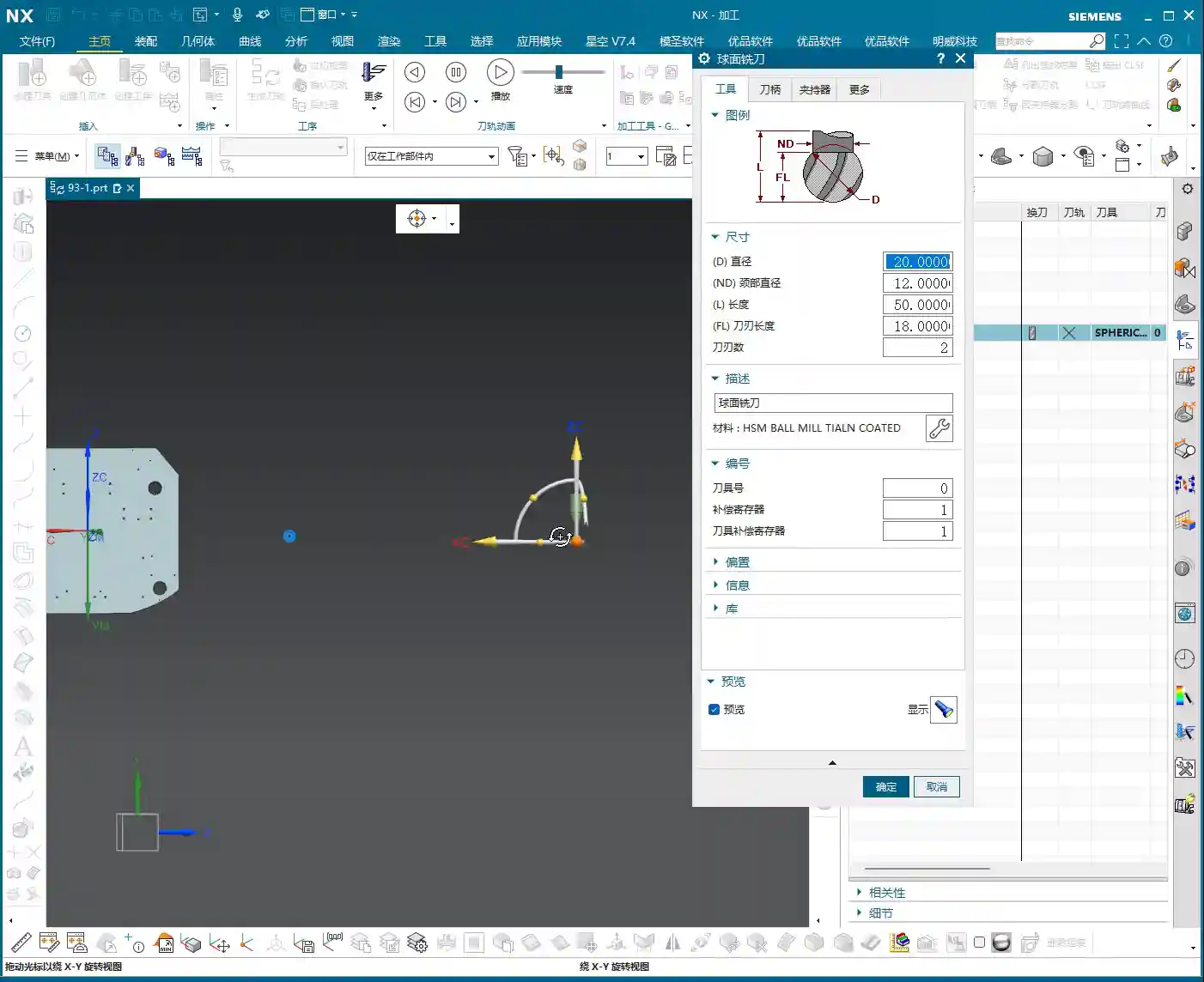
For the Guide Curve operation, we’ll use a D6 ball end mill this time. First, select the first guide curve, then the second. It’s that simple; nothing complicated.
After the program generates, you’ll notice a problem: this retract move (the pink rapid move lines in the program) is retracting excessively high, which is a huge waste of time! The machine running idle costs money! This needs to be fixed!
The height of this retract move is directly related to the stock distance parameter. Let’s reduce it, for example, to 1mm (approx. 0.04 inch). Recalculate, and see? It’s much lower now, isn’t it? Idle cutting time is instantly saved – that’s efficiency! Don’t underestimate these one or two millimeters; over years, the accumulated cost savings are significant.
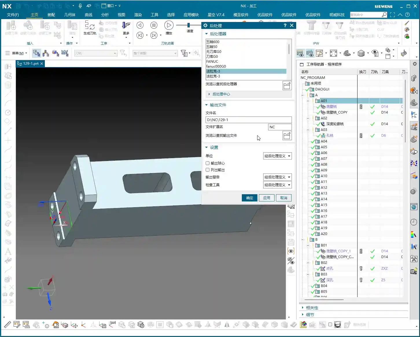
Final Checks and Program Transformation
All right, by now, all of our finishing pass programs are complete.
Overcut Check: The Last Line of Defense Before Machining
Next, overcut checking – this is absolutely mandatory every time. See, no alarms means no overcuts. If there were, the software would definitely throw an error. Never skip this step, or you’ll be devastated if the part is scrapped!
Simulation and Saving: Preventing Software Crashes
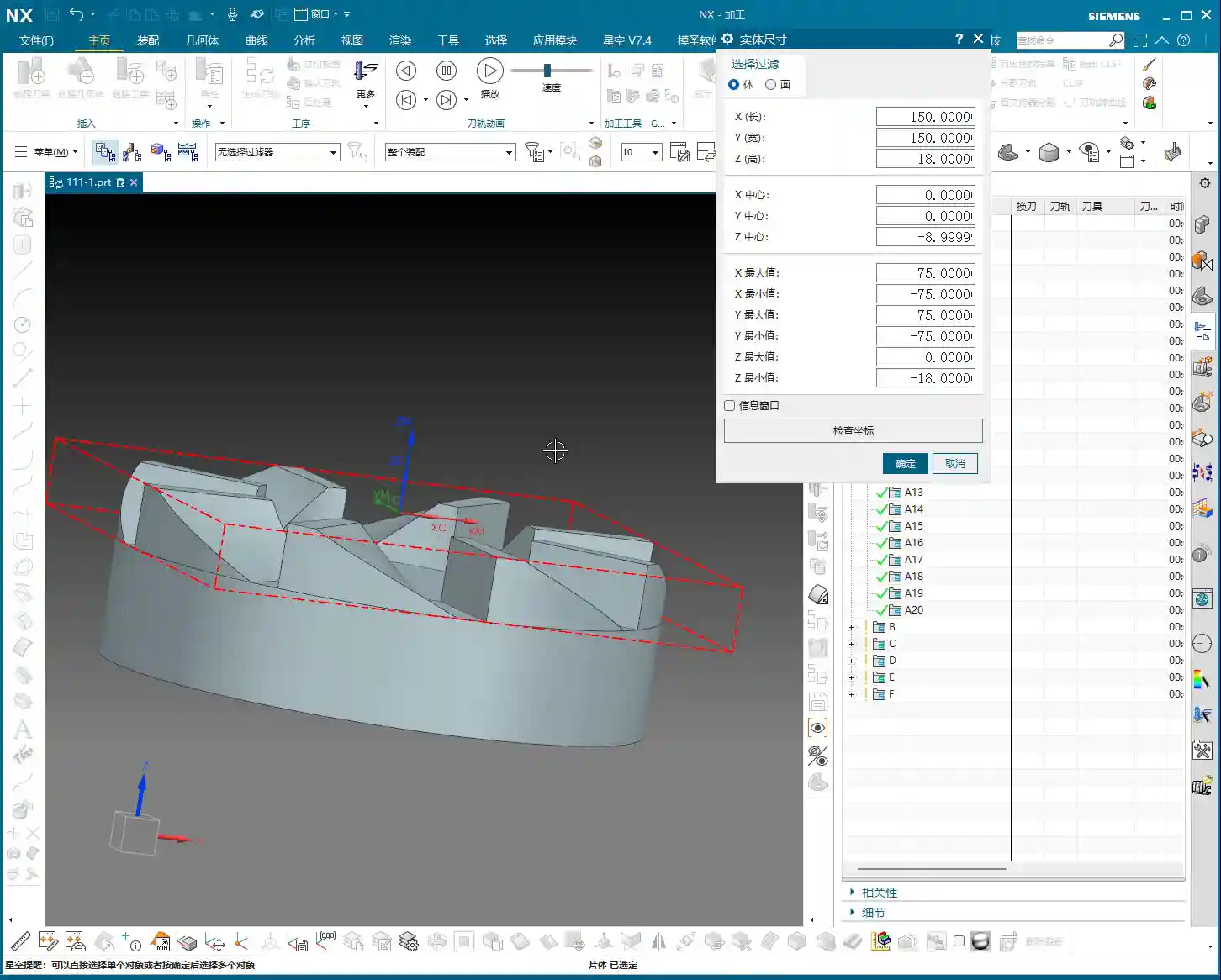
Then, save it! Remember, develop good habits. Sometimes, simulating directly can crash the software, leaving you with nothing. These are lessons learned the hard way. After saving, let’s simulate and check the results!
The simulation might not look absolutely perfect, especially with a D6 flat end mill (meaning a sharp corner/R0 tool); some details might not display completely. However, the actual machined part will be fine. I’ve machined these types of parts before with excellent results. These examples I share with you are all from parts I’ve actually machined. With that, this part is now complete.
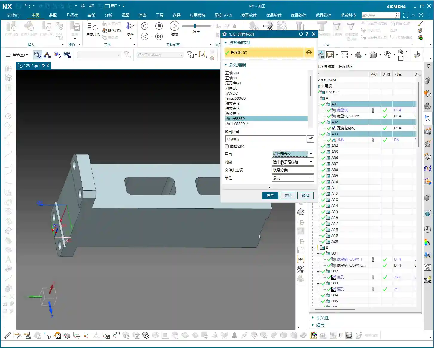
Program Transformation (Mirroring)
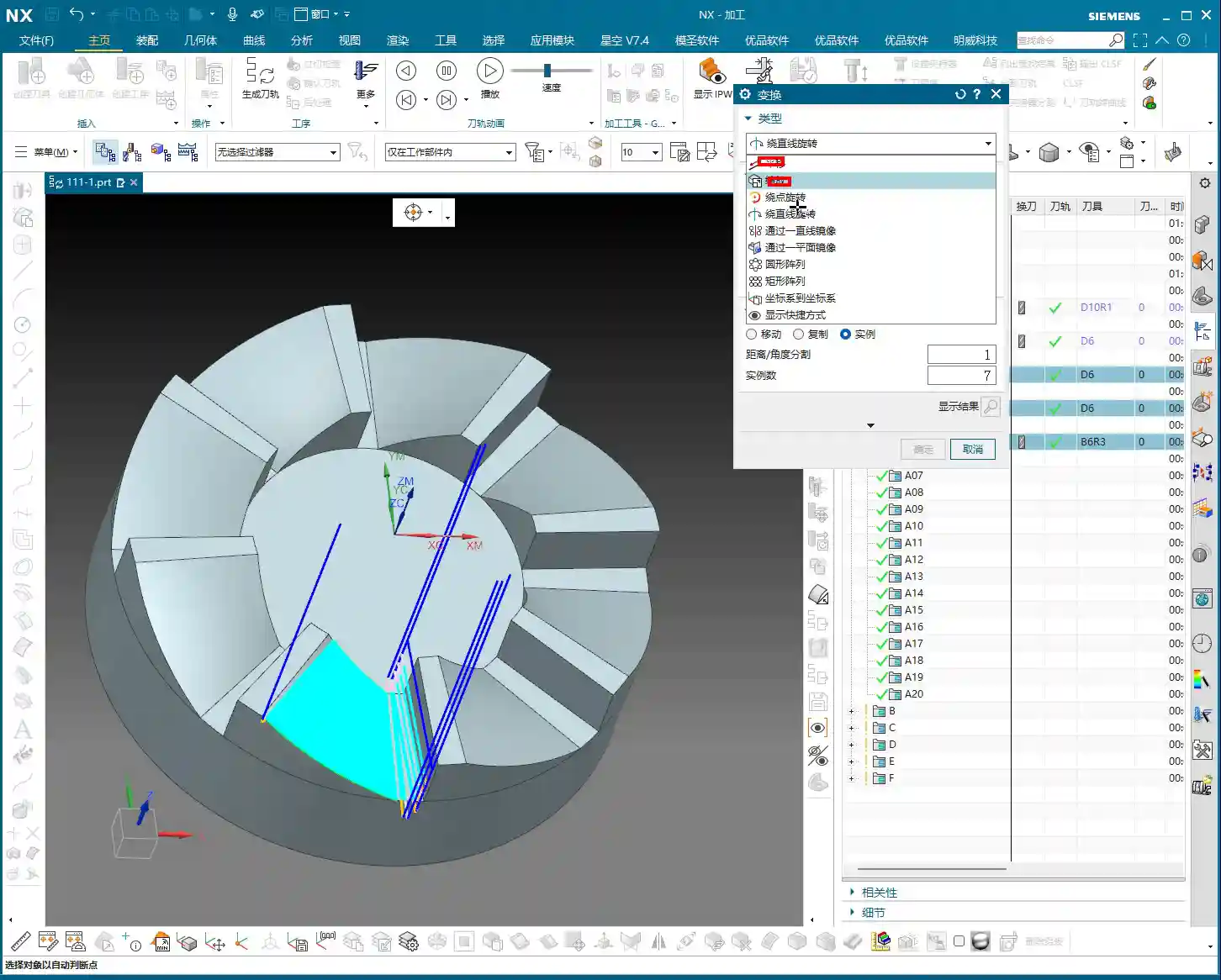
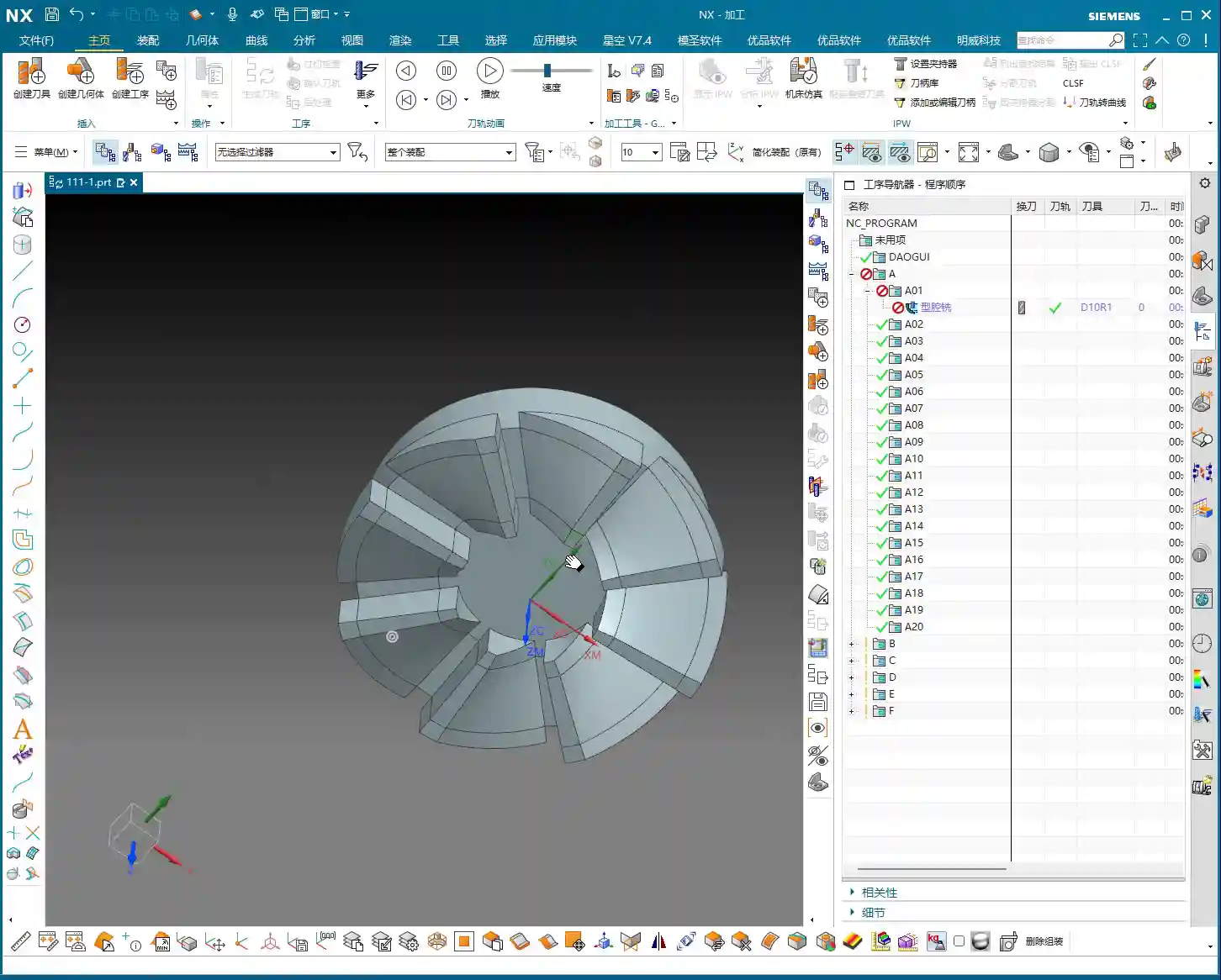
Final step, don’t forget to transform your previous roughing programs, meaning mirror them. This part is symmetrical, so some programs won’t require transformation, such as the side wall and bottom surface finishing passes. However, the corner cleanup might. Select the transformation object – it’s a simple task. With that, a complete set of machining programs for this rotary part is all done!
Summary: Pitfall Avoidance Guide
- Depth of Cut (DOC) Control: Divide the final 1mm (approx. 0.04 inch) of stock into multiple cutting layers; never take it off in a single pass, as this risks chatter or tool breakage, affecting surface finish.
- Rapid Move Optimization: Disable direct plunge-style rapid moves. Set a safe retract move height (retract to the stock surface) via “Non-Cutting Moves” to prevent collisions.
- Machining Area Simplification: When toolpaths exhibit abnormal behavior (failing to generate or excessive detours), check and simplify the selection of “Machining Areas” to avoid unnecessary restrictions.
- Corner Cleanup Tooling and Strategy: For corner cleanup, a flat end mill combined with Surface Drive is preferred; Guide Curve only supports ball end mills and is unsuitable for root corner cleanup.
- Precise Toolpath Trimming: Make good use of “Surface Percentage” to precisely control the start and end points of the toolpath, avoiding idle cuts or machining unnecessary areas.
- Retract Move Height Optimization: Adjust the “stock distance” parameter to reduce unnecessary retract move heights, saving idle cutting time and improving machining efficiency.
- Overcut Checking: Always perform an overcut check after generating each program; this is the final line of defense for ensuring part quality.
- Timely Saving: Before performing simulations or complex operations, cultivate the habit of saving frequently to prevent software crashes from causing data loss.
[VIDEO_HERE]
[EXCERPT] Hello everyone, this is Master Wang. Last time, we covered roughing. This time, the focus is on finishing rotary parts. From side walls to bottom surfaces, and then to root corner cleanup, I’ll walk you through programming efficient, high-quality toolpaths using Siemens NX. I’ll share practical tips you won’t find in textbooks, such as how to optimize tool retractions, prevent overcutting, and tackle various machining challenges. My goal is for you to not just program, but truly understand the machine and the process.
Step One: Finishing Side Walls and Bottom Surfaces – Refined Application of Depth Profile Milling
Listen up, last time we thoroughly covered roughing and semi-roughing. This time, we’re heading straight into finishing, focusing on the part’s side walls and bottom surfaces. Especially that bottom area – we might have left some stock last time, but this time it needs to be completely cleaned, leaving no blind spots.
Practical Tool Selection and Machining Area Definition
First, open your NX software. We’ll select a “Depth Profile Milling” operation. For tooling, we’ll directly choose our commonly used D6 flat end mill; this tool will handle the corner cleanup and side walls. As for the machining area, you can initially box-select the entire part; that’s fine, we’ll precisely define it later.
Hold on, what we need to do is specifically select these two areas: the side walls and the bottom surface. Remember, precision selection is better than broad selection. This avoids many unnecessary issues and computational load, improving program generation efficiency.
Depth of Cut and Multi-Pass Strategy
This program is primarily for finishing passes on the side walls. As I mentioned last time, the stepover for side walls should be tighter to achieve a smoother finish. For the bottom surface, we’ll machine down to a depth of -18mm. Of course, to be safe, you can adjust it slightly shallower, say -17mm, to leave a bit of stock for the final finishing pass.
Here’s the critical point: that last 1 millimeter (approx. 0.04 inch) of stock on the bottom surface (for example, from -17mm to -18mm) – you absolutely cannot take it off in a single pass! Doing so risks chatter or tool breakage, and the resulting surface won’t be flat. We need to split it into multiple layers, for instance, taking 0.3mm (approx. 0.012 inch) per Depth of Cut (DOC). By cutting in two to three layers this way, the cut will be stable, and the finish will be superior. Don’t just rely on software simulation; pay attention to the cutting sparks and the actual forces on the tool!
Additionally, the top 5 millimeters (approx. 0.2 inch) of the side wall should also receive extra finishing passes to improve its flatness. During the finishing pass stage, we won’t leave any stock; it’s a direct one-pass finish.
Cutting Parameters and Safety Strategies
For the cutting order, we’ll select Depth First. As for stepover, a linear cut at 55% or 60% is fine; this depends on your tool’s strength and material properties. However, I typically disable extension to avoid unnecessary toolpaths.
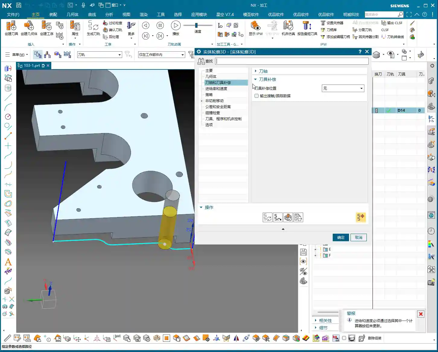
The program has generated, and the cutting depth control is fine. But look at this rapid move – it plunges directly into the side wall! This is unacceptable! A machine tool isn’t a computer simulation; this kind of move risks a collision. At best, you’ll scrap the tool and workpiece; at worst, you’ll damage the machine!
Therefore, we need to go into “Non-Cutting Moves” and modify the rapid transfer. For safety, retract to the stock surface; that 3-millimeter (approx. 0.12 inch) height is acceptable. This provides sufficient safe retraction space for the tool. This is a crucial safety procedure, remember that!
Here’s another trick: if the toolpath keeps failing to generate or takes excessive detours, it’s likely because a previously selected face is restricting it. Just select the bottom surface and the two side walls; don’t select the upper faces, let the tool move freely! Simplifying your selections often resolves major issues.
Finally, overcut checking is fundamental! Don’t assume everything is fine just because the program generated. One overcut can undo all your previous work, or even scrap the part.
Step Two: Corner Cleanup and Angled Surface Finishing – Surface Drive and Guide Curve
All right, the side walls and bottom surface are finished. Next, let’s address the root area of this part. After corner cleanup, we also need to perform contour milling on this angled surface. What command do you think is suitable?
Corner Cleanup Toolpath: Surface Drive is the Correct Approach
Some might think of using a “Guide Curve” for corner cleanup. But listen up: Guide Curve only supports ball end mills. How can a ball end mill perform corner cleanup? It simply can’t clean effectively! If the root has a sharp corner or small radius, a ball end mill can’t reach the bottom. Others might suggest using “Streamline” offset lines, which can also work, but that’s too much hassle—offsetting lines, selecting them—it’s highly inefficient!
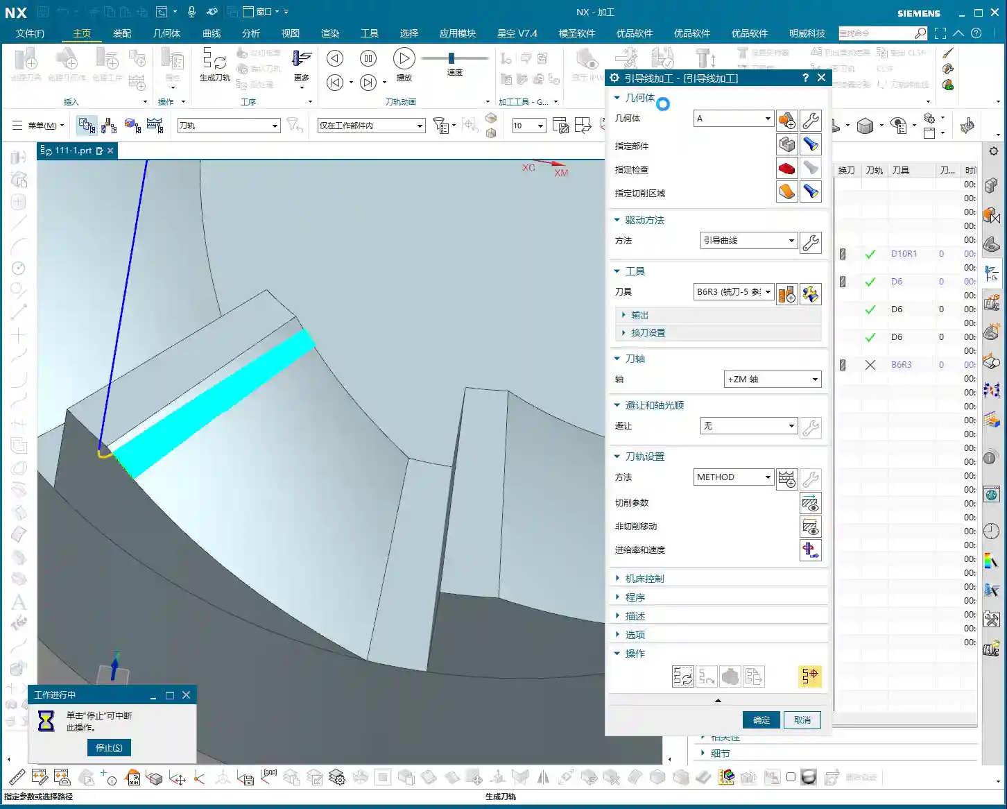
So, the most direct and effective method is our Surface Drive. This command is specifically designed for this! We’ll still use our D6 flat end mill. This time, there’s no need to select a machining area; just select the “drive face.”
Pay close attention to the cutting direction; we’ll set it to Material Reverse and use Zigzag machining for higher efficiency. For corner cleanup, a 0.1-millimeter (approx. 0.004 inch) stepover! When performing corner cleanup with a D6 flat end mill, a small stepover is crucial for a clean cut; otherwise, the finished surface won’t be flat, and all your effort will be wasted! Remember, finishing passes require attention to fine details; no need to change tolerances, just calculate the toolpath directly.
Toolpath Trimming: Precise Control of Machining Area
The program has generated, but it’s currently cutting from top to bottom, and we only need that small root area at the bottom. This is where the Trimming function comes in – listen up, this is key to boosting efficiency!
Within “Cutting Area,” locate “Surface Percentage.” See, we initially clicked this arrow (pointing at the direction), so Start Trim calculates from the top, and End Trim goes to the bottom. We need to shorten it to only machine the root area, which means modifying Start Trim. For example, changing it to 97% will make it cut only the very last portion. You’ll need to experiment a few times to find the appropriate percentage until the toolpath precisely covers the root area. This all comes from experience; you have to get hands-on.
Exploration: Applying Guide Curves and Optimizing Retract Moves
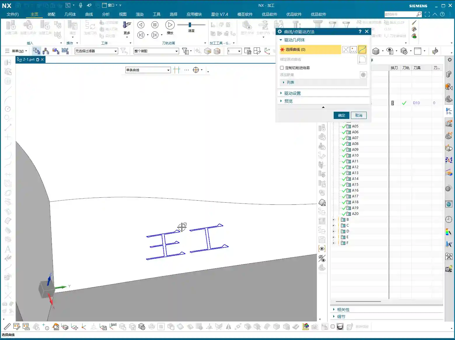
While Surface Drive works well for corner cleanup, to broaden your understanding of different methods, we can also try using a Guide Curve to machine this angled surface. You might not have used it much before, so let’s get some hands-on practice. Honestly, for machining such surfaces, any command will do – Contour Milling or Surface Drive, both are viable. The key is to find what’s best for the current situation; don’t fret, nothing is too difficult!
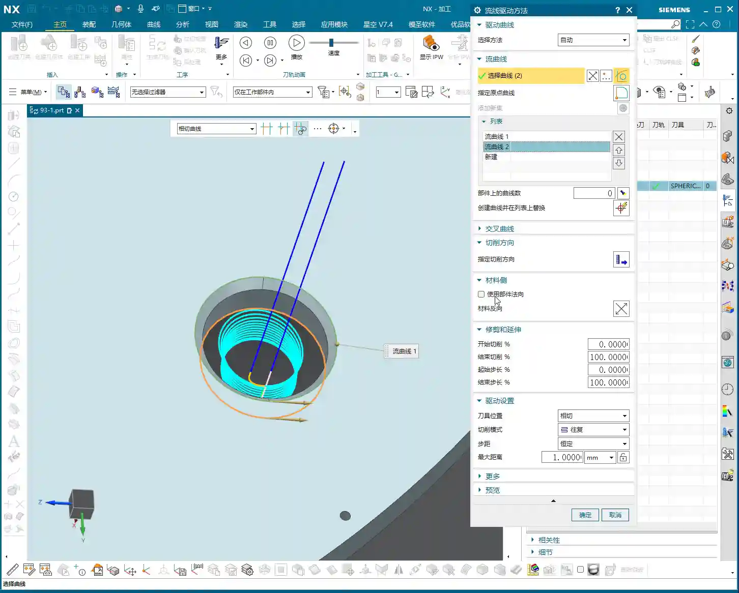
For the Guide Curve operation, we’ll use a D6 ball end mill this time. First, select the first guide curve, then the second. It’s that simple; nothing complicated.
After the program generates, you’ll notice a problem: this retract move (the pink rapid move lines in the program) is retracting excessively high, which is a huge waste of time! The machine running idle costs money! This needs to be fixed!
The height of this retract move is directly related to the stock distance parameter. Let’s reduce it, for example, to 1mm (approx. 0.04 inch). Recalculate, and see? It’s much lower now, isn’t it? Idle cutting time is instantly saved – that’s efficiency! Don’t underestimate these one or two millimeters; over years, the accumulated cost savings are significant.
Final Checks and Program Transformation
All right, by now, all of our finishing pass programs are complete.
Overcut Check: The Last Line of Defense Before Machining
Next, overcut checking – this is absolutely mandatory every time. See, no alarms means no overcuts. If there were, the software would definitely throw an error. Never skip this step, or you’ll be devastated if the part is scrapped!
Simulation and Saving: Preventing Software Crashes
Then, save it! Remember, develop good habits. Sometimes, simulating directly can crash the software, leaving you with nothing. These are lessons learned the hard way. After saving, let’s simulate and check the results!
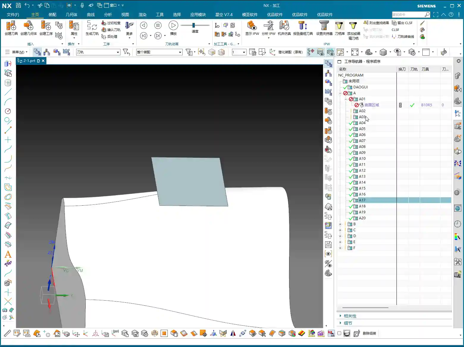
The simulation might not look absolutely perfect, especially with a D6 flat end mill (meaning a sharp corner/R0 tool); some details might not display completely. However, the actual machined part will be fine. I’ve machined these types of parts before with excellent results. These examples I share with you are all from parts I’ve actually machined. With that, this part is now complete.
Program Transformation (Mirroring)
Final step, don’t forget to transform your previous roughing programs, meaning mirror them. This part is symmetrical, so some programs won’t require transformation, such as the side wall and bottom surface finishing passes. However, the corner cleanup might. Select the transformation object – it’s a simple task. With that, a complete set of machining programs for this rotary part is all done!
Summary: Pitfall Avoidance Guide
- Depth of Cut (DOC) Control: Divide the final 1mm (approx. 0.04 inch) of stock into multiple cutting layers; never take it off in a single pass, as this risks chatter or tool breakage, affecting surface finish.
- Rapid Move Optimization: Disable direct plunge-style rapid moves. Set a safe retract move height (retract to the stock surface) via “Non-Cutting Moves” to prevent collisions.
- Machining Area Simplification: When toolpaths exhibit abnormal behavior (failing to generate or excessive detours), check and simplify the selection of “Machining Areas” to avoid unnecessary restrictions.
- Corner Cleanup Tooling and Strategy: For corner cleanup, a flat end mill combined with Surface Drive is preferred; Guide Curve only supports ball end mills and is unsuitable for root corner cleanup.
- Precise Toolpath Trimming: Make good use of “Surface Percentage” to precisely control the start and end points of the toolpath, avoiding idle cuts or machining unnecessary areas.
- Retract Move Height Optimization: Adjust the “stock distance” parameter to reduce unnecessary retract move heights, saving idle cutting time and improving machining efficiency.
- Overcut Checking: Always perform an overcut check after generating each program; this is the final line of defense for ensuring part quality.
- Timely Saving: Before performing simulations or complex operations, cultivate the habit of saving frequently to prevent software crashes from causing data loss.
👤 About the Author:
The author is a veteran CNC machining professional with 15 years of industry experience, specializing in UG NX programming. This article is an original work representing personal practical insights.
⚠️ Copyright Notice: Unauthorized reproduction or distribution without prior communication is strictly prohibited.